4.4Estimating Demand with a Public Transport Model
The best way to predict the future is to invent it.Immanuel Kant, philosopher, 1724–1804
Aggregating boarding, alighting, and customer flows, as in the previous section, provide a useful “first cut” approach to demand estimation. However, this data does not provide information on where people wish to travel. In most cases, a new BRT system will make changes in bus routes, and knowing the origins and destinations of trips (as opposed to boarding and alighting) is important to ensuring that the new services are closely aligned with where customers want to go. In particular, full OD information can inform the design of direct services that reduce the need for customers to transfer from one line to another. As a BRT system expands into a multi-route system, there will be many opportunities to significantly improve services and system efficiency by modifying routes and services, and the potential financial savings should more than pay for the additional cost and trouble associated with building a robust public transport model. This requires two new elements: the construction of a trip matrix and a route-choice model.
This section will describe how to build a basic transport model that models only the public transport system. With this basic public transport model, it will be possible to develop a much more robust estimate of the demand on the existing system. It will also enable the planning team to much more easily test the demand for different alternative scenarios for fares, as well as to optimize operational characteristics.
In many cities, some sort of transport model will already exist. But these models have generally been created for a specific purpose, and the purpose has rarely been to design a BRT system. Sometimes, existing models were designed for highway or transport departments and are only usable for motor vehicles, with very limited information on the public transport system. Others may have been created for building a metro, and not usable without additional work. Data is also far too often of poor quality. If a good quality transport model already exists, it should be possible to simply put the public transport system and the proposed BRT scenario into the existing model. However, in most cases the BRT team may have to start nearly from scratch. The public transport system should be modeled first, as this will be the most important information for BRT planning.
4.4.1Choosing a Modeling Software
The first step in setting up a public transport model is to obtain transport-modeling software. The development of transportation modeling software has greatly aided the process of transport supply and demand projections. Software models today can greatly ease the modeling process and increase accuracy and precision. But with the array of software products on the market, the transport planner can be left with an overwhelming set of options. Of course, there is no one software solution that is inherently correct. A range of variables will guide the software selection process. These variables include cost, familiarity of municipal staff and local consultants with a particular product, degree of user friendliness sought, degree of precision sought, and the overall objectives of the modeling task. The table below lists a few commonly used software packages on the market today.
Table 4.2Options for Transport-Modeling Software
| Software Name | Vendor | Comments |
|---|---|---|
| EMME | INRO | Good general purpose |
| CUBE | Citilabs | Good general purpose |
| TransCAD | Caliper Corporation | Good integration with GIS, easy to use |
| Visum | PTV | Good general purpose |
| QRS II | AJH Associates | Low cost but weaker on PT assignment |
| TMODEL | TModel Corporation | Low cost but weaker on PT assignment |
| SATURN | Atkins-ITS | Good for meso-simulation for congested vehicle assignment, but no PT assignment |
| AIMSUN 6 | Transport Simulation Systems | Integrated package for micro, meso, and macro simulation model |
| TRANUS | Free software developed by Modelistica | Integrated land use – transport model |
| Paramics | SIAS | Microsimulation package with integration capabilities |
| VISSIM | PTV | Microsimulation package, good animations, good integration with VISUM |
The strongest packages for general-purpose planning and design of BRT systems are EMME, CUBE, and VISUM, with TransCad offering close capabilities. All of these are expensive packages. However, in actuality, the most significant costs will be training staff to become familiar and adept with the software package. Older and more-sophisticated modelers, like the flexible Emme, allow staff to easily write subprograms, called “macros.” More and more consultants are now using Emme in combination with other programs with better GIS capability or with micro-simulation facilities. SATURN is a meso-simulation package that efficiently models groups (platoons) of vehicles and treats delays and congestion accurately, but its public transport facilities are too weak for BRT design. Equally, TMODEL and QRS II are weak at modeling public transport demand and are not recommended for BRT.
TRANUS can model land use and transportation systems. The transportation model can be used separately and is easy to use and calibrate. The land use model might be difficult to use and calibrate, particularly if many land uses are included in the modeling. Paramics and Vissim simulate trip making at a high level of detail, in particular vehicle-by-vehicle, and in some instances include pedestrians and traffic lights. These are very powerful packages for studying priority at junctions and interactions and delays at stops. They should only be used for these purposes and in combination with the macro demand models listed above, as they are not appropriate for BRT-route analysis. AIMSUN 6 is an integrated package that combines these micro-simulation features with micro- and macro-modeling facilities.
4.4.2Defining the Study Area and the Zoning System
Normally, the study area for a BRT system will be the areas currently served by bus and minibus services. If the decision maker has already preselected a particular corridor as the first BRT corridor, then the catchment area for this corridor will be the study area, but this may produce a lower demand forecast.
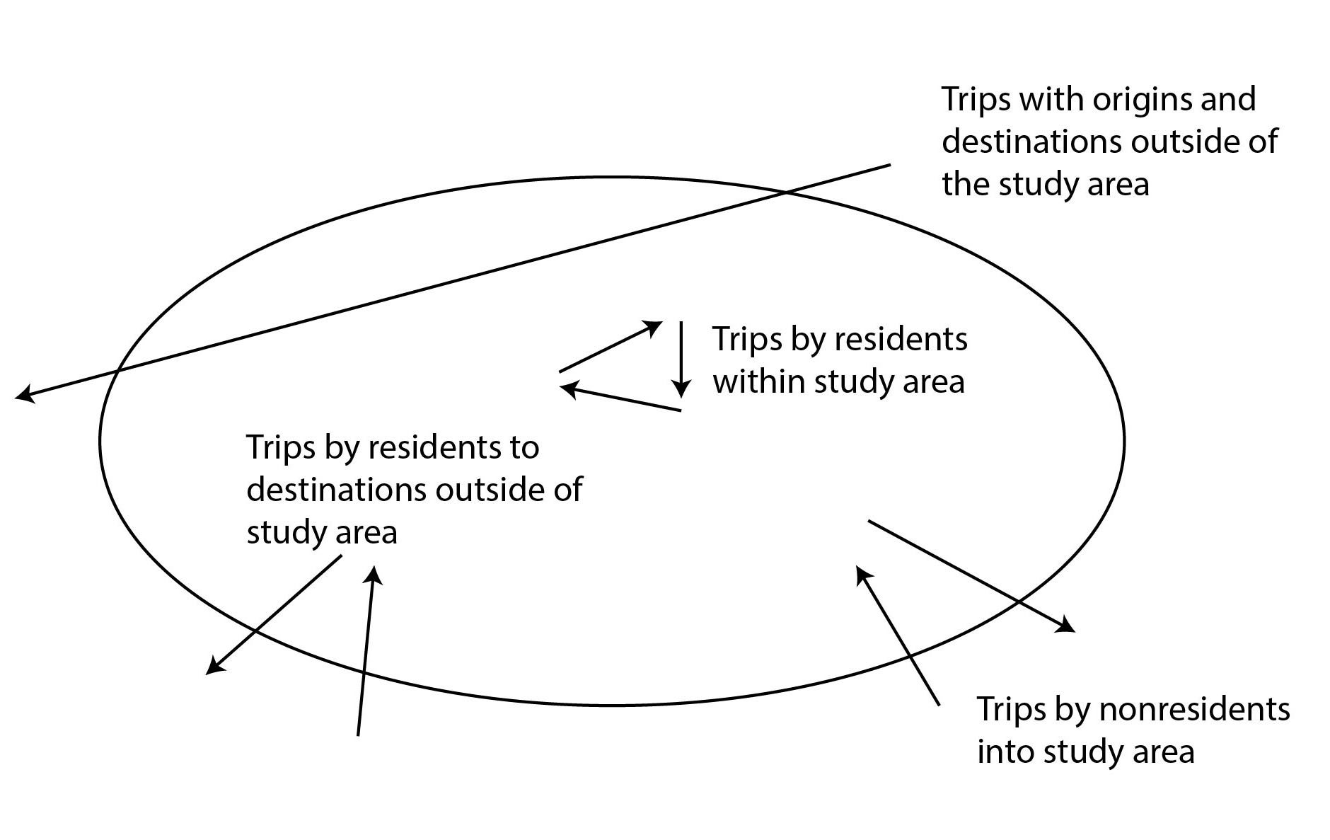
To analyze travel, the entire study area, as well as some locations outside the study area, need to be divided into a number of zones (Figure 4.22). As all origin-destination data will be collected and coded into this zoning system, establishing these zones is an important first step. Usually the zones are based on census tracts or political subdivisions that have been used as the basis of any existing census information or previous origin-destination studies. Using census and other administrative zones that already exist in the city will increase the chance of compatibility with the overlaying of different data types.
The information needed for modeling, however, is not exactly the same as the information needed for the census, so some census zones are usually consolidated into bigger zones or broken up into smaller zones. Transport modelers are generally less concerned about information outside the study area. As a result, they tend to consolidate zones outside the study area into fewer, larger zones. This consolidation is a simple matter of adding up the data associated with each zone.
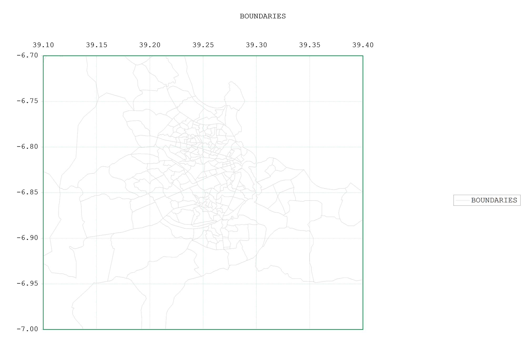
Typically, modelers need more-detailed information in the city center and/or along the proposed BRT corridor and its catchment area. So modelers will typically break up census zones into smaller zones, using more-detailed census data if available, or just dividing the zones using their judgment based on aerial photographs (Figure 4.24). Sometimes, households and employment will be concentrated into some parts of a large zone and not others, and it is important to break up the zone to capture this geographic concentration.
.
Selecting the size of the zones and the number of zones is a trade-off between accuracy, time, and cost. The size and number of zones will also depend in part on how the data was collected and how it will be used. Ideally, one would like to have a single zone associated with each BRT station/stop. However, this is not always feasible and some compromises are needed. For BRT systems in large cities like Jakarta and Bogotá, roughly five hundred and eight hundred zones, respectively, were used to analyze the main relevant BRT corridors. In a smaller city like Dar es Salaam, only three hundred zones were necessary for the main BRT-corridor analysis, though for detailed traffic-impact analysis, the city center was later broken down into an additional twenty zones.
Table 4.4 lists the number of zones that have been developed for various cities. Note that cities such as London have multiple levels of zones that permit both coarse- and fine-level analyses.
Table 4.3Typical Zone Numbers for Modeling Studies
| Location | Population | Number of Zones | Comments |
|---|---|---|---|
| Bogotá (2000) | 6.1 million | 800 | BRT project |
| Jakarta (2002) | 9 million | 500 | Strategic planning zones |
| Dar es Salaam (2005) | 2.5 million | 300 | BRT project |
| London (2006) | 7.2 million | 2252 | Fine level subzones |
| ~1000 | Strategic planning zones | ||
| Santiago (2009) | 5.5 million | ~700 | Strategic planning zones |
| Montreal Island (2008) | 3.4 million | 1425 | Strategic planning zones |
| Dallas-Fort Worth (2004) | 6.5 million | ~4900 | Strategic planning zones |
| Ahmedabad (2009) | 5.4 million | 1,400 | One zone per bus stop |
| Pune-Pimpri Chinchwad (2011) | 5.3 million | 1,855 | One zone per bus stop |
Source: Ortúzar and Willumsen (2011) and ITDP
Usually, models provide a good level of accuracy for trunk routes, but not necessarily for feeder routes. Feeder routes typically serve an area within a zone, especially outside of the direct catchment area of the BRT, where zones are normally a bit larger. Thus, those movements are not recorded in the model. A very detailed model to account for feeder routes, however, is not practical; so, besides using the modeling tool, the feeder system should be designed based on the existing system (field observation and experience) and allow flexibility to make changes during implementation.
These zones, and the road network, must be coded into the transport model. This process will not be described here in any detail, as it is a standard function of all transport modeling and is thoroughly described in the documentation of any commercially available transport demand model. The basic points of this process are summarized below.
Data is usually entered into a transport model either as a point, called a “node,” which has a specific “x” and “y” coordinate, or as a “link,” which is a line connecting two nodes. Normally, each intersection and each major bend in a road are assigned separate nodes. Nodes are usually numbered. Ideally, the x and y coordinates of each node should correspond to the actual latitude and longitude of that node. Making sure these nodes correspond to actual latitude and longitude is called “geocoding.” Geocoding will ensure that data from different sources are consistent.
Normally roads are broken up into different links. Links are usually named from their origin node and their destination node.
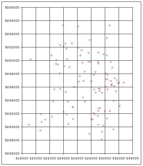
For example, in Dar es Salaam, there was already an existing GIS map. If no GIS map exists, then staff can utilize a GPS device to record the coordinates of each of these points (Figure 4.25). In Dar es Salaam, the team initially defined 102 nodes, and later increased it to 2,500 important nodes. By the end, the nodes represented most of the important intersections in the city. Each node was recorded in a simple spreadsheet (Table 4.5). Alternately, the street network can be traced over a geo-referenced aerial photo.
Table 4.4Node Coordinates in Dar es Salaam
| Node identification number | X coordinate | Y coordinate |
|---|---|---|
| 13 | 16340 | 26375 |
| 14 | 16835 | 26370 |
| 17 | 17212 | 26440 |
| 23 | 16433 | 26090 |
| 24 | 16835 | 26090 |
| 27 | 17339 | 26185 |
| 28 | 17580 | 26300 |
| 33 | 16435 | 25810 |
| 34 | 16835 | 26805 |
| 127 | 17110 | 26060 |
| 128 | 17540 | 25930 |
| 134 | 17285 | 25675 |
By connecting these nodes, a series of links are defined that represent different roads. For example, in Dar es Salaam, Morogoro Road between Sokoine Drive and Samora Avenue, is a link (the link between the nodes Morogoro Road X Sokoine Drive and Morogoro Road X Samora Avenue). Link data can also be entered into the transport model from an Excel spreadsheet (Table 4.6).
Table 4.5Link Data for the Transport Model in Dar es Salaam
| Link | Node A | Node B | Two directional |
|---|---|---|---|
| 1 | 13 | 14 | Yes |
| 2 | 14 | 17 | Yes |
| 3 | 13 | 23 | Yes |
| 4 | 14 | 24 | Yes |
| 5 | 17 | 27 | Yes |
| 6 | 23 | 24 | Yes |
| 7 | 24 | 127 | No |
| 8 | 127 | 27 | No |
| 9 | 27 | 28 | No |
| 10 | 23 | 33 | Yes |
| 11 | 24 | 34 | Yes |
| 12 | 33 | 34 | Yes |
| 13 | 28 | 128 | No |
| 14 | 128 | 134 | No |
| 15 | 134 | 34 | No |
These links are generally further defined based on the number of lanes, direction of movement, and other characteristics. However for public transport planning it is not really necessary to further define at this point.
Zones are generally entered into a transport model based on the nodes of all points that are needed to define the boundary. In an Excel spreadsheet, each zone will just look like a series of nodes defined by their x and y coordinates.
Once the data is entered into a model, the zone is actually represented by a special type of node called a “zone centroid.” This zone centroid is a node that is used to signify the average characteristics of the particular zone. In Dar es Salaam, for example, in addition to 2,500 nodes along roads, there were another 300 zone centroid nodes. Trips are generated and attracted to these centroids. It is therefore important to know how these centroids are connected in particular to stations in a new BRT design. Normally these zone centroids are in the middle of the zone, but if all the population is concentrated in one smaller part of a zone, it is better to move the zone centroid closer to the population concentration.
4.4.3Origin-Destination Survey and Matrix
There are two basic ways to create a public transport system origin-destination matrix for public transport customers without doing a household survey. The most common approach is to conduct an onboard origin destination survey of an entire study area. This survey is one of a family of surveys called intercept surveys, where individuals in the process of making a trip are interviewed either on a bus or minibus, or while riding their bicycle, about their trip origin and destination (where they began their trip and where they will end the trip) and also often the purpose of the trip. Planners should remember that this type of survey will not provide estimates for possible mode shift for private vehicles nor induced demand. And if it only applies to a portion of the city, it may not take into account important changes in travel patterns in the public transport system when a BRT system is implemented.
Another approach that is becoming popular, as mentioned in Section 4.3.5. above, is to do a type of boarding and alighting survey where customers are given a numbered token when boarding a bus or minibus, and then they turn in their token when alighting. In this way, their precise boarding and alighting location is recorded. This creates an OD matrix that is specific to a bus route. When all the bus-route-specific OD matrixes are added up, one has a type of OD matrix that has one main problem: it is unable to distinguish between those customers whose origin and destination are near the bus stop where they boarded or alighted, and those customers who are transferring to some other public transport route or other means of travel. This problem can be partially corrected by conducting extensive transfer surveys at any likely transfer point, and using the transfer ratios to adjust the OD matrix. This method is often faster, cheaper, and easier to conduct, and as a result larger sample sizes are usually viable. There is also a reduced risk of coding errors. It also has its downside. If the transfer points are not very well known, or if buses do not stop in regular locations, many transfers may be missed, leading to distortions. This sort of survey also does not provide useful information about trip purpose, and precise destinations that may be quite far from bus stops.
Origin-Destination is not always used by transport agencies to forecast ridership. According to a survey conducted for a Transit Cooperative Research Program (TCRP) report on forecasting and service-planning methods, only 29 percent of transport agencies in the United States consider OD data to be a major part of demand estimation. Nearly half (43 percent) consider OD data when forecasting ridership but do not see it as a major part of demand estimation. Twenty-three percent of agencies did not consider OD data at all.
Overall, the survey found that 63 percent of transport agencies used OD data gathered from onboard surveys and 40 percent of agencies used OD data derived from modeling as a source when forecasting ridership. In comparison, ridership data collected from fare boxes and by ride checks were much more likely to be used. Eighty-six percent of agencies used data from the fare box and 80 percent used occupancy surveys. Ridership data collected by automated customer counters, a relatively new means of data collection, was used by 40 percent of agencies. Other data sources considered were: existing land use patterns (71 percent), forecast land use patterns (54 percent), census demographic data (66 percent), and economic forecasts (31 percent) and trends (29 percent).
Data Collection for Intercept Survey Approach
All the origin and destination information collected will be coded as between the zone centroids of two of these zones, and aggregated based on these zones. A trip between two zones is called an “origin-destination pair,” or OD pair. The table of all the trips between each OD pair by any given mode, in this case public transport, is called the OD matrix.
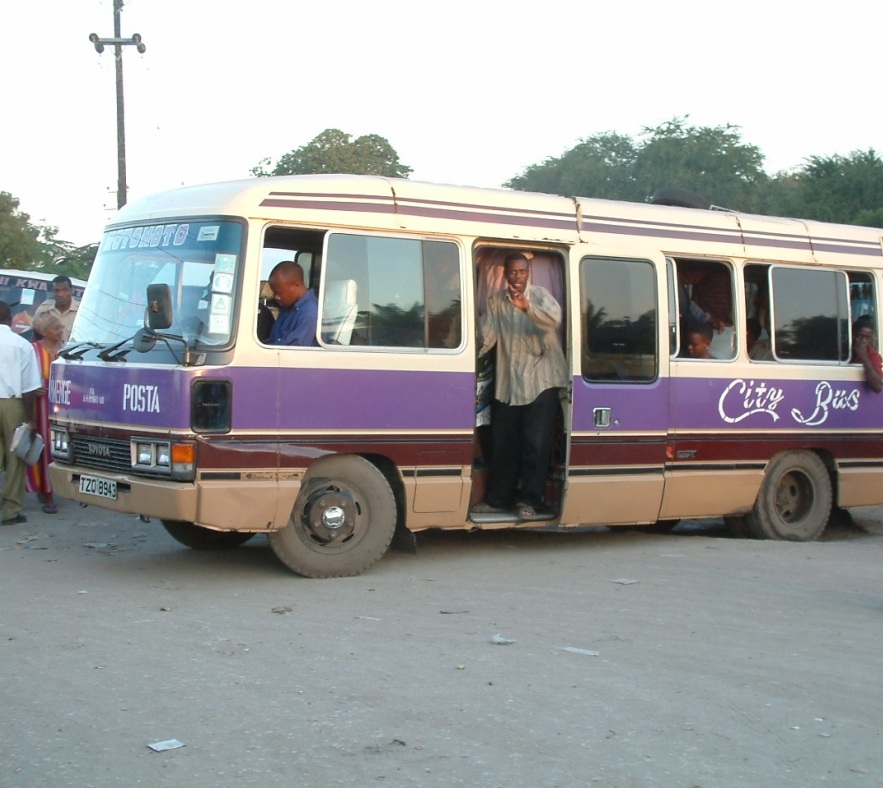
To conduct an onboard OD survey, public transport users are interviewed either on board a bus or minibus vehicle (in that case it is not an interception point, but a section of a road between two intersections) or at stops and interchanges. Sometimes, with the cooperation of the police, minibus customers can be interviewed very efficiently by having the van driver pull over and allow the customers to be interviewed. In Dar es Salaam, with the cooperation of the police, the planning team, wearing DART (Dar es Salaam Rapid Transit) shirts, stopped Daladalas (paratransit vehicles) and interviewed all of the customers inside (Figure 4.24). Other data besides OD information can also be collected, if appropriate. Other useful information can include the fares paid and the services used, but the questions should be kept as simple as possible. Although it is tempting to ask about waiting times, these are seldom accurately reported by individuals and are best estimated by another method.
Onboard OD surveys of bus customers typically attempt to focus on customer flows during the morning peak period. However, it can be difficult to avoid capturing nonpeak trips as well, so normally data is collected for approximately four hours around the morning peak, and averages are taken or weighted.
The survey locations should correspond to the locations where the traffic counts were conducted earlier, if these points were chosen wisely. In the case of Dar es Salaam, the points where the OD surveys were conducted were the same thirty-four points of the original traffic counts. This precision was possible due to the assistance of the police in pulling over vehicles at particular locations. In Jakarta, the surveys were conducted on board the buses and minibuses, so surveys were conducted along key links that corresponded as closely as possible to the points where previous traffic counts had been conducted.
Sample Size
The sample size for intercept surveys depends on the accuracy required and the population of interest. The error for an intercept OD survey is a function of the number of possible zones that a customer might travel when passing through a particular point. As a simple rule, Ortúzar and Willumsen (2011) suggest the following table for a 95 percent confidence, with a margin of error of 10 percent for given customer flows:
Table 4.6Sample size for origin-destination surveys
| Expected Customer flow (customers/period) | Sample size (percent) |
|---|---|
| 900 + | 10 percent |
| 700–899 | 12.5 percent |
| 500–699 | 16.6 percent |
| 300–499 | 25 percent |
| 200–299 | 33 percent |
| 1–199 | 50 percent |
Usually, on potential BRT corridors, the flows are much greater than 900, so 10 percent of the total customer flow at any given survey point is a reasonable rule. In the case of Dar es Salaam, the average customer flow at the peak hour was 10,000, so 1,000 customers were surveyed at each point, or some 34,000 surveys for all the points. In Jakarta, 120,000 surveys were conducted, but only about 65,000 of the surveys were usable. This quantity was all that was possible with the budget available, and constituted roughly 3 percent of the peak hour flows. In Jakarta, the survey numbers were weighted based on the flows on the corridor.
Origins and destinations should be recorded as accurately as possible—for example, as the nearest intersection or other key identifier. These locations then have to be attributed to the zone in which they are located, so the origin and destination can be coded to the zone centroids.
Error Types
The data collection process is prone to two types of errors: measurement errors and sampling errors. Measurement errors arise from misunderstandings and misperceptions between the questions asked and the responses of the sampled subjects. Misinterpretation by the interviewer can result in the incorrect listing of a response. Frequently, during an OD survey, for instance, a person will identify the origin and destination of their trip, but neither the interviewee nor the surveyor are able to locate this location within any of the zones on a map. Sometimes surveyors will also not do the work responsibly and will make up answers. There may also be a degree of bias in which respondents answer questions in a manner that represents a desired state rather than a reality.
Avoiding measurement errors is a complex process that requires a lot of local knowledge, and should start at the survey stage. One method is to ask the interviewee the best local landmark, and have the local staff identify as precisely as possible its location on a map. Another method is to have the interviewees pick their origin and destination from a preselected list of areas and subareas, and specific popular destinations. The latter method will probably avoid a lot of trouble and confusion, but will lose some subtlety regarding walking distances. In countries where street names and neighborhoods are far from standardized, the latter method may be more effective.
Sampling errors occur due to the cost and feasibility of surveying very large sample sizes. Sampling errors are approximately inversely proportional to the square root of the number of observations, i.e., to halve them it is necessary to quadruple the sample size.
Origin Destination Matrixes
Once each OD pair is coded to specific zone centroids, a separate OD matrix is created for each survey point. For each survey point and each direction, it is simply a matter of adding up the trips surveyed between each OD pair for the peak hour. This raw survey data will give you a preliminary OD matrix for each direction at each survey point. Table 4.8 outlines the general form of a two-dimensional trip matrix.
Table 4.7General form for a two-dimensional trip matrix
| Origins | Destinations | |||||
|---|---|---|---|---|---|---|
| 1 | 2 | 3 | …j | …z | ∑j Tij | |
| 1 | T11 | T12 | T13 | …T1j | …T1z | O1 |
| 2 | T21 | T22 | T23 | T2j | T2z | O2 |
| 3 | Tij | Tij | Tij | Tij | Tij | O3 |
| I | Ti1 | Ti2 | Ti3 | Tij | Tiz | Oi |
| Z | Tz1 | Tz2 | Tz3 | Tzj | Tzz | Oz |
| ∑i Tij | D1 | D2 | D3 | …Dj | …Dz | ∑ij Tij = T |
Source: Ortúzar and Willumsen 2011.
From Table 4.8, “T11” indicates how many trips were made within Zone 1; “Tij” indicates the total surveyed trips between Zone i and Zone j; “O1” is the total origins in Zone 1, and “D1” is the total destinations in Zone 1.
This simple matrix is still not a full OD matrix for the whole city’s public transport trips during the peak hour. To get to that, the number of people surveyed needs to be related to the total number of public transport customers per direction per hour at each survey point. This process is called expanding the matrix. The total number of public transport customers at the peak hour is taken from the data that was collected earlier at each of the same points using the public transport vehicle-occupancy surveys. For example, in Dar es Salaam, on some corridors 1,000 out of 10,000 hourly public transport customers per direction were collected on some corridors, which yielded an expansion factor of ten. On this matrix, the observed OD trips need to be multiplied by ten to get the total public transport trips at the peak hour. On other corridors, where 1,000 interviews were taken for only 6,000 customer flows, the expansion factor is six, so the surveyed OD trips need to be multiplied by six. Each separate matrix needs to be expanded by its appropriate expansion factor (as indicated in Table 4.9.), or can be expanded using a single expansion factor.
Table 4.8OD Matrixes Expanded by Expansion Factor
| Point | Initial factor | Sample | PAX/Peak Hour | Daladala small | Daladala large |
|---|---|---|---|---|---|
| P01W1 | 12.9295302 | 298 | 3853 | ||
| P01W2 | 1.53046595 | 558 | 854 | ||
| P02W1 | 6.545655774 | 493 | 3227.008297 | 320.5 | 63 |
| P03W1 | 5.833990702 | 515 | 3004.505212 | 68 | 68 |
| P03W2 | 2.928214064 | 522 | 1528.527741 | 60 | 54 |
| P04W1 | 14.87864833 | 619 | 9209.883319 | 409.5 | 95.50 |
| P06W1 | 9.375530401 | 511 | 4790.896035 | 65.5 | 107 |
| P06W2 | 4.431338691 | 358 | 1586.419251 | 83 | 62.5 |
| P07W1 | 2.597194766 | 502 | 1303.791773 | 164 | 8 |
| P07W2 | 9.968302596 | 449 | 4475.767865 | 210 | 16 |
| P09W1 | 12.92116263 | 470 | 6072.946436 | 180.5 | 65.5 |
| P09W2 | 6.609650125 | 485 | 3205.680311 | 181 | 47.50 |
| P10W1 | 25.42999509 | 515 | 13096.44747 | 628.5 | 65.5 |
Because the point of each OD survey was chosen to pick up a discrete set of OD pairs, each individual OD matrix will largely cover a different part of the city, but there will be some overlap and therefore the risk of “double counting” trips will happen twice. The individual matrices will have some OD pairs with actual values, and some OD pairs with zero trips (Tables 4.10 and 4.11).
Table 4.9OD Matrix #1 Eastbound Morogoro Road and United Nations Intersection
| Origins | Destinations | |||||
|---|---|---|---|---|---|---|
| 1 | 2 | 3 | 4 | 5 | ∑j Tij | |
| 1 | 4 | 10 | 6 | 0 | 0 | O1 |
| 2 | 12 | 4 | 2 | 0 | 0 | O2 |
| 3 | 16 | 5 | 12 | 0 | 0 | O3 |
| 4 | 3 | 2 | 0 | 0 | 0 | Oi |
| 5 | 0 | 0 | 0 | 0 | 0 | Oz |
| D1 | D2 | D3 | D4 | D5 | Total |
Table 4.10OD Matrix #2 Southbound Old Bagamoyo Road and United Nations Intersection
| Origins | Destinations | |||||
|---|---|---|---|---|---|---|
| 1 | 2 | 3 | 4 | 5 | ∑j Tij | |
| 1 | 0 | 0 | 0 | 12 | 15 | O1 |
| 2 | 0 | 0 | 3 | 15 | 20 | O2 |
| 3 | 5 | 2 | 15 | 8 | 10 | O3 |
| 4 | 0 | 0 | 0 | 6 | 11 | Oi |
| 5 | 0 | 0 | 5 | 12 | 10 | Oz |
| D1 | D2 | D3 | D4 | D5 |
To develop the full OD matrix for public transport trips in Dar es Salaam, a simple estimate would be to take the maximum value for any OD Pair in any observed survey. Strictly speaking, the correct value for each cell where multiple observations are expected depends on \(p_{ij}^a\), the proportion of trips between origin \(i\) and destination \(j\) that pass through each intercept point \(a\), on \(r_a\), the sampling ratio at each point \(a\) (a number between \(0\) and \(1\)), and on \(s_{ij}^a\), the number of trips between \(i\) and \(j\) observed at point \(a\). Then, the correct estimator for the number of trips when there are \(n_{ij}\) points that would have intercepted trips from \(i\) to \(j\), is:
\[T_{ij} = \frac{\displaystyle\sum_{n_{ij}} \frac{s_{ij}^a}{r^a}}{\displaystyle\sum_{n_{ij}} p_{ij}^a}\]
Of course, if there is only one intercept point for that OD pair (\(n_{ij} = 1\)) and there is only one useful route from \(i\) to \(j\) (\(p_{ij}^a =1\)), then the formula reverts to the familiar sample expansion:
\[T_{ij} = \frac{s_{ij}^a}{r^a}\]
For illustration purposes in Table 4.12, the values from the previous two tables have been combined to form a complete OD matrix (assuming that only two points are surveyed).
Table 4.11OD Matrix Dar es Salaam
| Origins | Destinations | |||||
|---|---|---|---|---|---|---|
| 1 | 2 | 3 | 4 | 5 | ∑j Tij | |
| 1 | 4 | 10 | 6 | 12 | 15 | O1 |
| 2 | 12 | 4 | 3 | 15 | 20 | O2 |
| 3 | 16 | 5 | 15 | 8 | 10 | O3 |
| 4 | 3 | 2 | 0 | 6 | 11 | Oi |
| 5 | 0 | 0 | 5 | 12 | 10 | Oz |
| D1 | D2 | D3 | D4 | D5 | Total |
This methodology is used to avoid the double (or triple) counting of some trips. This double counting may happen because some journeys may have been intercepted by more than one survey station, either potentially or in the sample. In this case, steps must be taken to avoid exaggerating their importance in the matrix by weighting those cells appropriately—for example, taking the average value of duplicated cell entries. On the other hand, people may go in very different directions to reach the same endpoint, so using this method will undercount the total demand. For more details, consult Ortúzar and Willumsen 2011.
Validation
Due to these distortions, along with measurement and sampling errors, it is usually necessary to undertake corrective actions. A validation process is typically done at the conclusion of the data-collection process in order to provide a degree of quality control.
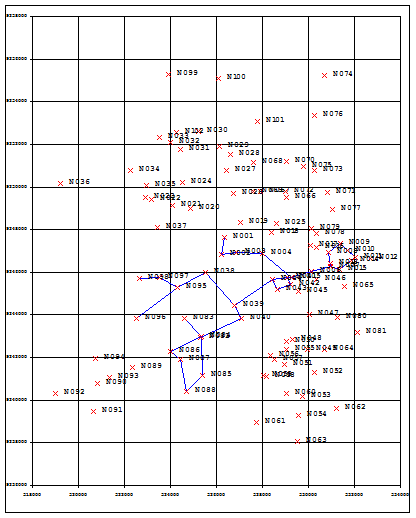
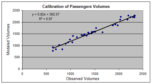
Validation is usually accomplished by looking at OD pairs route by route, and doing an informal trip assignment, assigning the OD trips to specific public transport routes, and comparing the aggregate total trips to the aggregate trip counts developed from the occupancy surveys and public transport vehicle counts (Figure 4.27).
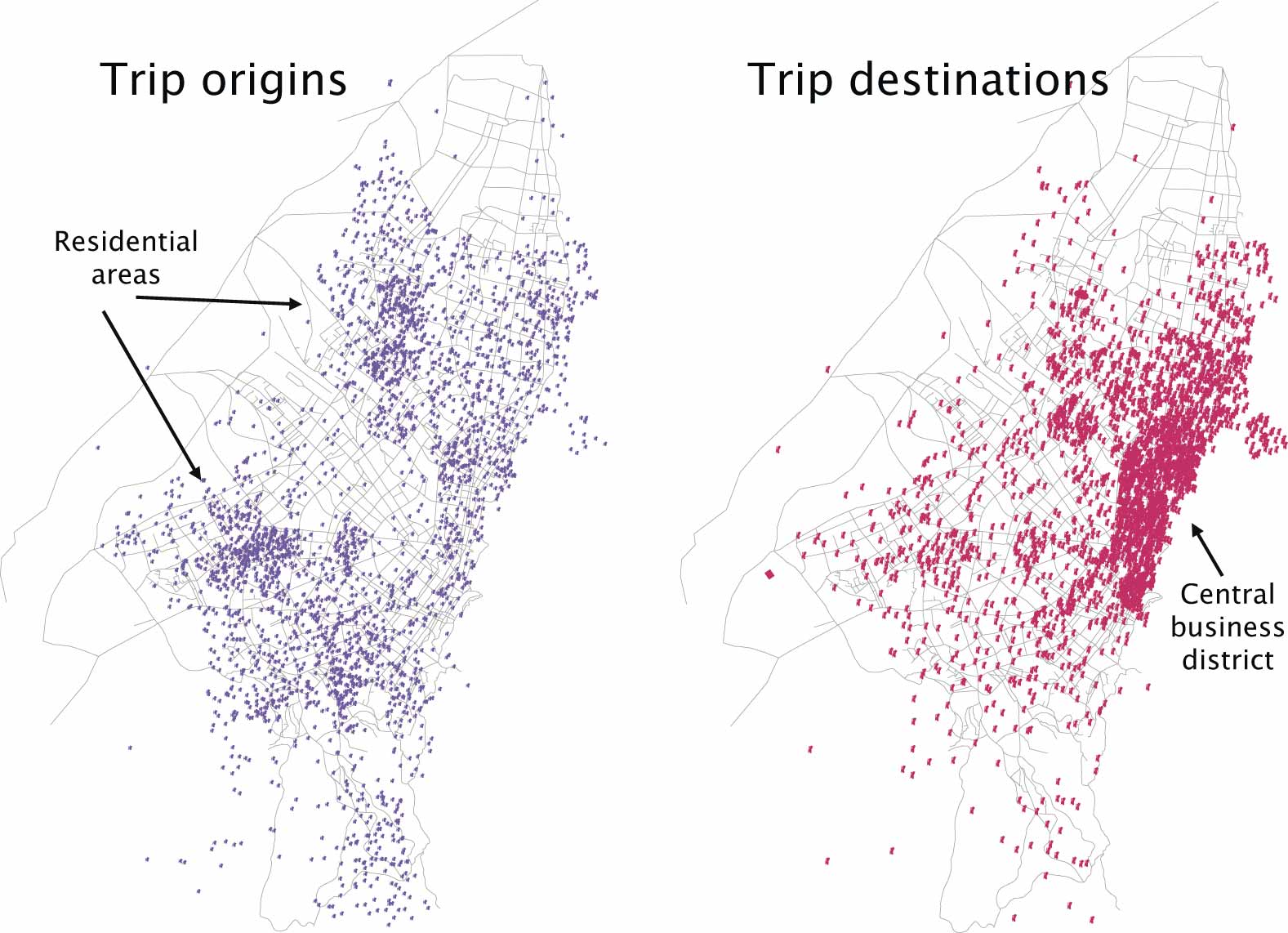
Once the OD matrix has been cleaned and calibrated, the OD matrix can be input into the transport model, and the testing of different scenarios can begin. The OD matrix can also be used to generate an origin-destination map that gives decision makers an overall view of the density of origins and destinations in the city. The OD map will frequently illustrate the extent to which trips are distributed or are centralized within the city. The OD map of Bogotá shows that there is a heavy concentration of trip destinations to the central business district (Figure 4.28).
4.4.4Outputs of the Public Transport Model
Once the road system and the OD matrix are input into the transport model, different scenarios for the BRT system can be tested. While the output from the public transport model will be used at various points throughout this guide, for the time being it will be used to generate demand estimates for specific BRT system scenarios.
The first step is generally to take a look at the existing public transport demand on all major corridors throughout the city at the peak hour. These results should now yield a much more accurate estimate of total existing public transport demand on all the major corridors in the city. This result is a valuable tool for prioritizing which corridors should be included in the BRT system. Figure 4.29 is a picture of the total existing public transport demand on all of the major corridors in Jakarta.
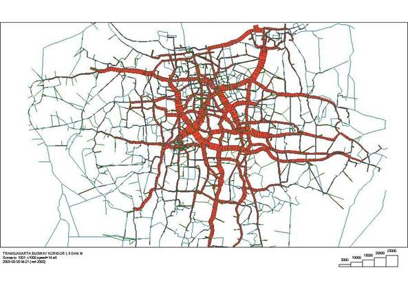
These total-demand estimates, or “desire lines,” tell how many public transport customers are currently on each major corridor. It still does not say anything about how many public transport customers will be on a specific BRT system.
When first coding the existing public transport system into the model, the following additional information will be required:
- Vehicle capacity (total standing capacity is all that is used);
- Public transport (this will be a series of links; each direction needs to be coded separately because sometimes bus routes do not go and return on the same roads);
- Specific location of the bus stops (for most of the network, just assume the bus stops are at the intersections, but the BRT corridor nodes should be added specifically at the bus stop, and the links between the bus stops should be broken into separate links);
- Speed on each link (this will be taken from the bus speed and boarding and alighting survey);
- Bus fare (usually the models allow fare distance, and if there is a flat fare leave the distance blank);
- Bus frequency;
- Value of time (there are various ways of calculating this value, but in practice this value is based either on interviews with bus customers or typically 50 percent of the hourly wage rate for the typical bus customer).
At this point, the scenario to be tested should be carefully defined. In the case of TransJakarta, the scenario was essentially defined through a decision taken by the governor. The governor’s design decision was as follows:
- TransJakarta would go from Blok M to Kota station with twenty-four stops at specific locations;
- TransJakarta would have fully segregated lanes and of certain design;
- TransJakarta would charge a flat fare of Rp. 2,500 (US$0.30);
- There would be no feeder buses and no (functional) discount transfers from any existing routes;
- Ten existing bus lines travelling between Blok M and Kota would be cut; all other bus routes would be allowed to continue to operate in the mixed traffic lanes at curbside bus stops;
- Fifty-four buses were procured to operate in the system.
When coding this BRT scenario into the public transport model, there is a small difference between coding a new BRT link and coding just any other bus route. In order to test some unique elements of the BRT system, the BRT link will be coded as an entirely new road link with special BRT characteristics, rather than assuming that it is a bus line operating on an existing road link that is open to paratransit vehicles and other vehicles. This new BRT link in the model will only be coded for use by a specific BRT vehicle that may be a new vehicle category that does not already exist. In the case of Jakarta, these vehicles are only used on the BRT system. This special coding of the BRT link is also required to give this route special fare characteristics, such as the possibility of free transfers between routes when the system expands to more than one route. Thus, coding a new BRT route is no different from coding any public transport route, except:
- The bus speed will be higher than for routes on the mixed traffic links. The BRT bus speed must be calculated specifically based on the system’s design, but it is generally between 20 and 29 kph (see Chapter 6 for more information);
- Some new station locations will be created, which will affect walking times;
- Bus frequencies will be specific to the number of buses and the bus speed;
- If a lane of mixed traffic is being removed from the existing link, the definition of the characteristics of that link will need to be changed to reflect the loss of a lane. This change will only be necessary for running the full transport model in the future;
- It may be necessary to adjust the bus speeds downward for all the bus routes that are running in the mixed-traffic lanes. If there is only a public transport model, this will only be an estimated impact. If there is a full transportation-demand model, the model will help calculate this impact.
After defining the new BRT links and assigning them a new BRT route with the characteristics reflecting the political decision, the projected demand for this specific scenario can be calculated (Figure 4.30).
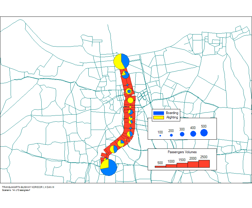
In the case of Jakarta, the projected demand on Corridor I for the scenario determined by the governor was tested. Based on the lack of a feeder system and the unwillingness to cut bus routes that ran parallel to the new BRT system, the demand on the new system would not be very high. Because one mixed traffic lane had been removed, while few of the buses in the mixed traffic lanes had been removed, mixed traffic lanes would be more congested. However, due to the lack of a full transport model, the precise scale of this impact was not known. The planning team therefore encouraged the governor to expand the trunk system rapidly, to add feeder buses with free transfers onto the trunk system, and to cut more existing parallel bus routes.
Note that this demand estimate assumed that the new BRT system would only get the trips from existing public transport trips. It did not assume that any trips would be attracted from other modes, as the public transport model alone did not have the capacity to provide much of an answer to this question. Nevertheless, this analysis produced a very good conservative first estimate of the likely demand.
To include some possible modal shift from private vehicles, one can usually use the same rough estimate methodology recommended in Figure 4.2 above. In Bogotá, where a well-designed system actually decongested the mixed traffic lanes, the modal shift impact in the first phase was a modest 10 percent of private-vehicle users to the BRT system. The shift came from both push and pull factors. Most directly, competing routes by existing operators were eliminated or moved to parallel corridors. As the system has expanded, approximately 20 percent of current BRT customers on TransMilenio are former private-vehicle users. In Jakarta, where few bus routes were cut but the level of service for mixed traffic was more adversely affected, the mode shift was higher, at around 20 percent from taxis, cars, and motorbikes. In Ahmedabad, India, where there were very few bus customers originally on the corridor, there was an even higher modal shift (less than 30 percent), mostly from motorized three-wheelers and motorcycles, which before accounted for less than 70 percent of the existing modal split.
With this demand estimate, planners are better able to assess whether the physical designs proposed will have sufficient capacity to handle the projected demand, whether stations will be congested, and whether or not the system is likely to be profitable or operate at a loss. Planners can optimize the proposed-route network to increase load factors and minimize the need for customer transfers.