4.6Risk and Uncertainty
Doubt is uncomfortable, but certainty is absurd.Voltaire, writer, historian, and philosopher, 1694–1778
However sophisticated, a model of transport demand is still a model, a simplified representation of a real-world scenario. A degree of uncertainty will always remain in any travel-demand forecast, and BRT planners should keep this in mind.
In terms of demand forecasting, there are two main sources of error:
- Will the variables that define the future context (population, income, location, employment, etc.) and policy environment (car restraint, competition, pricing, and subsidies) for the BRT adopt the values forecast at the planning stage?
- Do the models capture true travel behavior, and will the travel preferences identified (coefficients in the generalized cost formulation and the different sub-models) remain in the future?
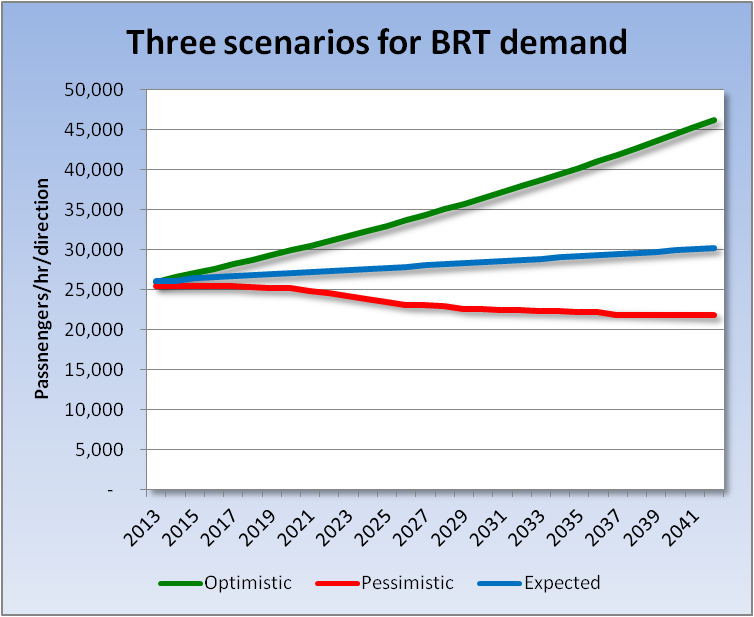
The best way to handle these sources of uncertainty is to develop forecasts under different scenarios. In the worst circumstances, more-dispersed urban growth will continue to incentivize the use of conventional buses, taxis, and minibuses and compete, to some extent, with the BRT system, and that no car-reduction policy will be implemented. In the best-case scenario, urban growth will be focused on BRT, car-reduction policies will be implemented, competing modes will be kept some distance away from the BRT trunk network, and they will not be subsidized. An expected or probable scenario would assume a partial implementation of those policies. The definition of these scenarios will have to be agreed upon by all stakeholders, with some consultation of possible bidders and financial institutions.
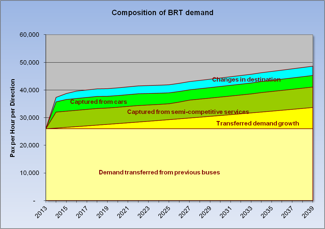
Uncertainties about capturing the true travel behavior within the model can be treated in different ways. While it is difficult for a model to accurately capture travel behavior, the basis for the model will be the demand on the existing routes that currently run on the corridor. Those existing routes and their combination of services are reasonably predictable. Ideally, that demand will have transferred to the new BRT corridor if those previous services are no longer allowed to run on the corridor and that should form the basis of any forecast. This transferred demand will tend to grow with population, although this is perhaps less certain.
Other components of BRT demand will be those captured from semi-competitive modes not fully removed from competition: taxis and shared taxis. Other demand may be abstracted from cars if the BRT service is good enough and car restraint policies are implemented. Finally, some people may choose to change the destination of their trips, perhaps for shopping or entertainment, to take advantage of the better accessibility offered by BRT.
These sources of demand have been outlined in increasing degrees of uncertainty or confidence in our ability to model them accurately enough. It is desirable, therefore, to present the final demand estimations and deconstruct the individual components or contributions. This is illustrated in Figure 4.35. In this way, private and public sector stakeholders, concerned about the sources of risk in the project, can understand the most solid basis for demand and revenue projections.
Finally, some stakeholders, particularly in the financial community, advocate the use of stochastic simulations to address the issue of uncertainty in forecasts. In this case, the analysis involves the use of Monte Carlo simulations usually implemented as an add-on to a standard spreadsheet.
The first step is to agree with stakeholders on the few input or model variables that will be considered stochastic rather than fixed, and relate the outputs from the model to the stakeholders. Additional model runs will be needed to identify, for example, how variations in GDP growth affect revenues and therefore car ownership. This requires exercising the model in sensitivity tests, using different values of time in mode choice.
The next step would be to adopt some probabilistic distribution around the mean expected values of these variables. It is common to assume that these would be independent normal distributions, although this assumption was partly to blame in the risk models before the 2008 financial crisis.
The next step is to construct a model where this handful of variables affects demand, and where their probabilistic distributions are sampled repeatedly in a Monte Carlo simulation. Each run of a Monte Carlo simulation reflects one possible demand and revenue path diverging from the expected scenario. This is illustrated in Figure 14.36, where each path represents a diversion from the expected case normalized to 1; a revenue factor value of 0.95 in one year implies that collections in that case would be only 95 percent of the expected case for that year.
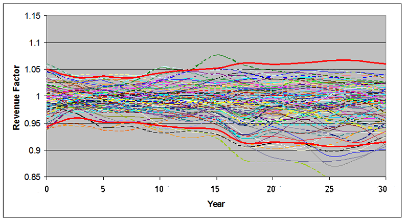
These results can be aggregated in different ways to express the probability that a particular level of demand (and revenue) will be exceeded, say, 90 percent of the time. This is usually referred to as the P90 forecast and it is sometimes used to finance private sector schemes.
The value of this treatment is limited in the case of BRT schemes where uncertainty resides more in transport and land use policy that is better treated through scenario analysis.