15.3Technical Fare and Customer Fare
But surely for everything you have to love you have to pay some price.Agatha Christie, writer, 1890–1976
15.3.1Calculating the Technical Fare
The total revenues distributed to the various contracted parties are based on the amounts collected from the system’s “technical fare.” The technical fare is equivalent to a flat fare that the system would be required to charge in order to break even. By contrast, the “customer fare” refers to the fare paid by the users of the system. As will be discussed in this section, the technical fare and customer fare are likely to be slightly different values.
The technical fare represents the actual cost per customer of providing the service. It is the basis for the subsequent distribution of revenues to the operators. It is calculated by simply adding up the full estimated operational costs calculated for the trunk operators, the feeder bus operators, the fare collection company, the trust fund manager, and the administration costs of the BRT authority (if the BRT authority costs are to be included). These operational costs include both the ongoing operational costs and any operational investments that will be the financial responsibility of the private investors, including the depreciation of the vehicle value and financing charges. The following equation summarizes this basic relationship.
Eq. 15.3 Basic form of technical fare calculation:
\[ \text{Technical fare} = {\text{cost}_\text{operational} \over \text{Customers}_\text{Daily} } \]
Where:
- \( \text{cost}_\text{operational}\): Total BRT system daily operational costs;
- \( \text{Customers}_\text{Daily}\): Total projected daily customers.
Figure 15.10 provides a more detailed and expanded calculation of the technical fare.
The contracts for the private operating companies are likely to be nonuniform. Some companies will invest only in ninety vehicles, while others will invest in more. In the case of TransMilenio, it was decided that there would be four trunk operating companies in the first phase. The number of vehicles purchased by the four different companies was: (1) 150 vehicles; (2) 120 vehicles; (3) 100 vehicles; and, (4) 90 vehicles. System planners estimated, based on projected demand, that each vehicle would operate roughly 247 kilometers per day, and they used this estimate as the basis of the calculation of the technical fare. Contractually, however, the operators were not guaranteed any minimum number of vehicle kilometers per day, or they would not have been exposed to any demand risk. Rather, they were guaranteed 850,000 vehicle kilometers within a 15-year period.
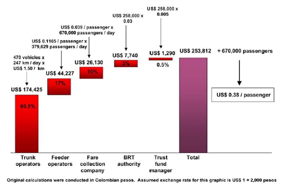
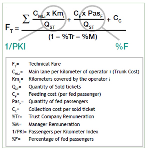
Because the operator is paid per vehicle kilometer, this meant that the cost of trunk operations to TransMilenio was the total number of vehicles times the total number of vehicle kilometers. The actual formula to calculate the technical fare is depicted in Figure 15.11.
The example given in 15.11 is specific to the first phase of the Bogotá TransMilenio system. Each system will have its own cost structure based on the amount of the service that is provided by the trunk line vehicles vis-à-vis the feeder vehicles, the fare collection costs, the negotiated service rates of each component, and the cost of administration. In the case of TransMilenio’s Phase I, 69 percent of the cost of operating the entire system resulted from payments to the trunk line operators, but this will be different for each system. This value also changed with the addition of the Phase II corridors in Bogotá.
The technical fare, calculated on a cost-plus basis from the overall operating costs of the system, is the basis for the distribution of fare revenues. In other words, each component of the TransMilenio system was promised a fixed percentage of the total fare revenues based on the calculation of the technical fare. In this way, these companies became shareholders with a collective stake in maintaining ridership.
15.3.2Adjusting the Technical Fare
An operator concession agreement will typically be in the range of ten years, the estimated life of a vehicle, though it could be shorter if the vehicles can easily be resold. During that period, many of the input costs can change (e.g., fuel costs, labor costs, etc.). Since the concession agreements stipulate that revenues are paid based on the vehicle kilometers travelled, both the BRT authority and the operators must be protected against dramatic changes in input cost levels.
The technical fare goes through a process of modification depending on cost swings in both system inputs and operational factors. Fuel price volatility is one of the most significant risks. Spare parts that need to be imported will be subject to currency risk, a major factor in some countries. Base labor costs will vary in step with the local economy. Accurately predicting these cost levels over a long period is a nearly impossible task due to the great number of external influences. Thus, as base cost conditions change for the operators, the technical fare will go through adjustments.
Table 15.3Factors Affecting Changes in the Technical Fare
| Category | Cost item |
|---|---|
| System inputs | Diesel price;; Consumer price index; Minimum wage standard;Producer price indexes (lubricants, tires, maintenance). |
| Operational factors | Passenger per kilometer index (PKI); Percentage of passengers using feeder services. |
On a periodic basis, such as every two weeks, the technical fare is updated based on the changes in the base factors. The calculation for the changes in the technical fare is given in Equation 15.4.
Eq. 15.4 Calculating changes in the technical fare:
\[ ∆F_T = \%C_{ML} {∆C_{ML} \over ∆PKI} + \%C_F (∆C_F + ∆\%F) + \%C_C ∆C_C - 1 \]
Where:
- \( ∆F_T \): Change in the technical fare;
- \( \%C_{ML} \): Proportion of the main lane cost (%);
- \( ∆C_{ML} \): Change in the cost per kilometer (main lane);
- \( ∆PKI \): Change in the passengers per kilometer (main lane);
- \( \%C_F \): Proportion of the feeder cost;
- \( ∆C_F \): Change in the feeder remuneration, by passenger that use feeding services;
- \( ∆\%F \): Change in the percentage of passengers that use feeding services;
- \( \%C_C \): Proportion of the collection cost;
- \( ∆C_C \): Change in the collection cost.
15.3.3Customer Fare and Contingency Fund
As noted above, the “customer fare” is the payment required by the customer for a single trip on the system. Unfortunately, costs tend to rise over time, implying that fares must also rise. For reasons of customer clarity, as well as political considerations, the fare paid by the customer should not be changed frequently, perhaps no more than once or twice per year. Customers would be quite confused and angry if the fare changed every time world fuel prices changed. Further, raising customer fares can have a range of social equity impacts that must always be considered. If a public transport company needs to obtain political approval for each fare increase, then the adjustments may never happen. In turn, the entire system will eventually become financially untenable.
To overcome such an inherent stalemate, the system for fare adjustments should be relatively automatic in nature, based on contractual obligations linked to key trigger points. TransMilenio has worked out a mechanism for adjusting the fare automatically to such changes. In the case of Bogotá, all operating costs are calculated on a biweekly basis. If a particular trigger point is reached, such as the technical fare exceeding the customer fare, then a fare adjustment is authorized by the municipality. The mayor and other political officials are still involved in the authorization through the public company’s board of directors, but the stipulation of a fare adjustment is reached through the operating cost calculation.
However, at the same time, some political discretion is required. As noted, fare level changes should not be frequent events. Also, it is probably sensible to establish fare levels that are round numbers in order to coincide with denominations of the local currency. For example, a fare of US$0.375 is not a possibility. Further, a fare level that requires handling many small coins means that both fare collection and fiduciary handling of the revenues will be slowed down. This inefficiency will in effect increase costs even more. Thus, fare levels should only increase at prescribed trigger points, and the increase should be significant enough so that no further increases will be likely over the short term. A fare adjustment system should be ideally designed so that increases do not occur more than once or twice per year.
If unusual events occur (e.g., hyperinflation) that require frequent adjustments, a contingency fund should be in place to bridge revenue shortfalls. The contingency fund thus provides a buffer that allows the system management company to stabilize fare levels even in turbulent times. It is this need for some buffer against unexpected contingencies that led to the development of a contingency fund in the case of TransMilenio. The difference between the technical fare in Bogotá and the customer fare is simply that an additional charge has been created to pay into a contingency fund (Equation 15.5).
Eq. 15.5 Relationship between customer fare, technical fare, and contingency fund:
\[ \text{Customer fare} = \text{Technical fare} + \text{Contingency fund payment} \]
Figure 15.12 graphically illustrates the relationship between the customer fare and the technical fare. In general, the customer fare should be slightly greater than the technical fare, and this difference is deposited into the contingency fund.
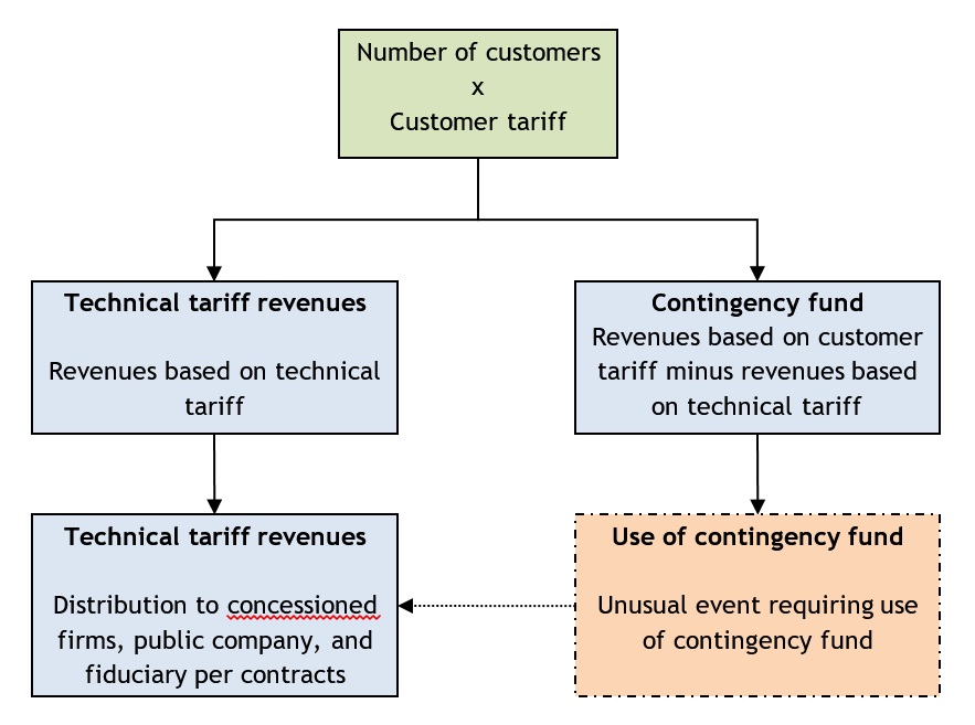
The contingency fund is designed to handle unexpected events such as unusual low levels of service demand, extended hours of operation, terrorism and vandalism, and problems associated with hyperinflation. In general, the customer fare will be greater than the technical fare, and thus the contingency fund will build up a positive balance. When unforeseen circumstances occur and the technical fare exceeds the customer fare, then proceeds from the contingency fund will be drawn upon for a temporary period. The contingency fund effectively acts as a safety net in times of unusual cost fluctuations. As the contingency fund becomes exhausted, the board of directors of the system will have to act in order to avoid a financial crisis.
The standard remedy would be to raise the customer fare to a point securely above the technical fare. The operation of the contingency fund provides a level of security and confidence to the operators as well as any outside funding entities to the system.
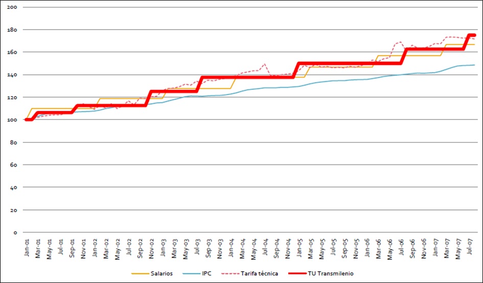
Figure 15.13 tracks the technical fare and the customer fare in the TransMilenio system. As expected, the customer fare is generally greater than the technical fare. As the technical fare has increased with time, the customer fare has also increased in order to maintain a comfortable margin. The graphic also demonstrates the difference in fluctuations between each fare type. The customer fare only increases in discrete amounts since these represent points of actual fare increases to the customer. By contrast, the technical fare will likely vary to some degree each month, as the constituent cost categories will change with economic conditions and input prices.
15.3.4Fare Elasticity
In general, elasticity is the degree to which a demand or supply curve reacts to a change in price. Elasticity is not a fixed value, and it varies among products and services depending on how essential they are to the customer. Products and services that are essential are less sensitive to price modifications because customers would continue buying these products despite price increases. Products that are not essential are more sensitive to price modifications; if the price rose too much, people would stop buying or consuming these products.
When it comes to transport planning, elasticities have several applications. They can be utilized to estimate the ridership and revenue effects of changes in public transport fares. They are also used in modelling to estimate how changes in public transport service will affect the vehicle traffic volume. And finally, they can be useful when evaluating the benefits and impacts of mobility management strategies such as new public transport services, road tolls, and parking fees, among others.
Some of the factors that affect public transport elasticities are summarized below:
- Trip Type: Non-commute trips tend to be more dependable on price changes than other kind of trips such as commute trips. Elasticities for off-peak public transport travel are typically 1.5 to 2 times higher than peak intervals elasticities. This is because peak-period travel largely consists of commute trips;
- User Type: Public transport-dependent riders are generally slightly less price sensitive than choice or discretionary riders (these are the people who own a car and can use it for that trip). Some demographic groups, including nondrivers, people with low incomes, people with disabilities, high school and college students, and elderly people are more likely to be more public transport dependent. Generally, public transport-dependent people are a relatively small part of the total population but a large portion of public transport users, while discretionary riders are a potentially large but more price elastic public transport market segment;
- Geography: Unlike suburbs and smaller cities, large cities tend to have lower price elasticities, because they have a greater portion of public transport-dependent users. This is due to increased traffic congestion and parking costs, and improved public transport service due to economies of scale.
Phil Goodwin, in the document “A Review of New Demand Elasticities with Special Reference to Short and Long Run Effects of Price Changes,” produced the average elasticity values summarized in Table 15.4. He noted that price impacts tend to increase over time as consumers have more options (related to increases in real incomes, automobile ownership, and now telecommunications that can substitute for physical travel). In 2006, Peter Nelson, Andrew Baglino, Winston Harrington, Elena Safirova, and Abram Lipman found similar values in their analysis of Washington, D.C., public transport demand.
Table 15.4Transportation Elasticities
| Short-Run | Long-Run | Not Defined | |
|---|---|---|---|
| Bus demand WRT fare cost | -0.28 | -0.55 | |
| Railway demand WRT fare cost | -0.65 | -1.08 | |
| Public transport WRT petrol price | 0.34 | ||
| Car ownership WRT general public transport costs | 0.1 to 0.3 | ||
| Petrol consumption WRT petrol price | -0.27 | -0.71 | -0.53 |
| Traffic levels WRT petrol price | -0.16 | -0.33 |
Source: Todd Litman, Victoria Transport Policy Institute.
One key thing to keep in mind is that no single public transport elasticity value applies in all situations. Various factors affect price sensitivities, including type of user and trip, geographic conditions, and time period. Available evidence suggests that the elasticity of public transport ridership with respect to fares is usually in the –0.2 to –0.5 range in the short run (first year), and increases to –0.6 to –0.9 over the long run (five to ten years). These are mostly affected by the following factors:
- Public transport price elasticities are higher for discretionary riders than for dependent riders;
- Elasticity values are about twice as high for off-peak and leisure travel as for peak and commute travel;
- Cross-elasticities between public transport and automobile travel are relatively low in the short run (0.05), but increase over the long run (probably to 0.3 and perhaps as high as 0.4);
- Due to variability and uncertainty, it is preferable to use ranges rather than point values for elasticity analysis;
- A relatively large fare reduction is generally needed to attract motorists to public transport, since they are discretionary riders. Such travelers may be more responsive to service quality (speed, frequency, and comfort), and higher automobile operating costs through road or parking pricing.
15.3.5Adjusting the Technical Fare
Whenever the BRT authority finds that the technical fare is too different from the expected fare (taking into account the different objectives of the system), the BRT authority can take the following actions in order to adjust the technical fare:
- Operational or logistical adjustments in the system;
- Reduction in operational expenditures. This means reductions in any of the items included in the technical fare shown in Section 15.3.1: Calculating the Technical Fare;
- Reduction of the level of service (pax/m2). This should be taken carefully since this could affect in a negative way the reputation of the system;
- Subsidies for Capex and/or Opex. In this point it is strongly recommended that the BRT authority chooses a subsidy that covers the Capex rather than an Opex one, so that the system does not have to incur in a monthly dependency from the subsidy to operate.
As has been suggested, setting the fare level requires analyzing two different values:
- The technical fare, or the fare needed for full cost recovery;
- The optimal customer fare, or the fare that maximizes the system’s profits.
Ideally, the business and operational model of the BRT system should bring the technical fare as close to the optimal customer fare as possible.