24.1Basic Concepts
Change means movement. Movement means friction. Only in the frictionless vacuum of a non-existent abstract world can movement or change occur without that abrasive friction of conflict.Saul Alinsky, political activist, 1909–1972
24.1.1About Intersections
The intersection is the area where two or more roads meet each other. The use of the word in Traffic Engineering technical language implies “roads for vehicles” and “at the same level,” but very often the expressions “at-grade intersections” or “single-grade intersections” are used to demonstrate the same concept. For flyovers and underpasses the term used is “interchange” or “separated-grade interchange.” When more than one mode is involved, the common traffic engineers’ wording is “crossing” as in “pedestrian crossing” (one of the roads is assumed to be a roadway); recently the term multimodal intersection has also been applied.
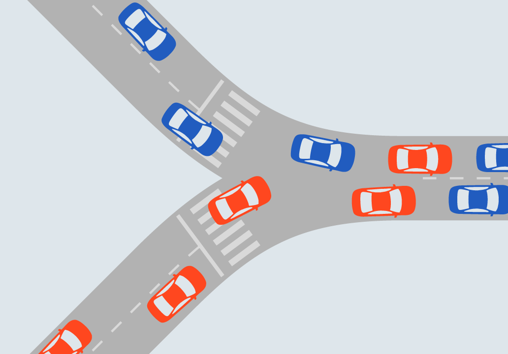
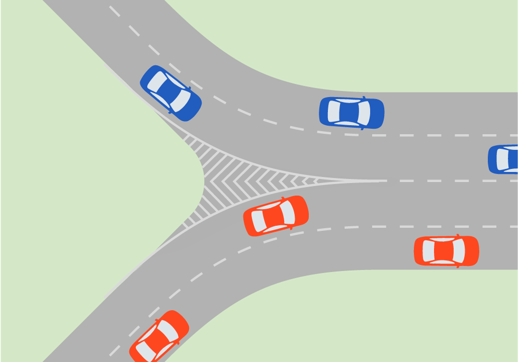
By this definition, an intersection implies conflicts of vehicles attempting to use the same space and can refer to a unidirectional T-shaped or Y-shaped confluence area. The conflict in this area becomes clear as there is not enough space to accommodate the two incoming flows as they move into the exiting stream in a congested situation (Figure 24.1). Conversely, a channeled Y-shaped junction may not be an intersection (Figure 24.2).
Because the majority of cases where two or more roads meet include many possible turning movements (not all conflicting), intersections can be seen as linking several other adjacent intersections as well—that is, an intersection is a larger conflict area that is composed of smaller conflict areas (or smaller intersections).
Footpaths (or “roads for people”) are more important to accessibility in populated areas, therefore roadways are usually constructed between footpaths. When two roadways meet, several walkway crossings are needed. So a multimodal intersection encompasses a larger area than just the roadways where people conflict in trying to use the same space. (To keep things in perspective, let us remember that drivers and passengers are people.)
The more conflicts there are in an intersection or in a crossing, the greater amount of time people will need to cross it safely. If there is a low frequency of vehicles arriving at the intersection where pedestrians, cyclists, or other vehicles want to cross, then those wanting to cross can do so safely without compromising travel time by what is known as “passage negotiation,” or waiting until the way is clear to cross. If over the years the vehicle frequencies throughout the day rise to the point where queues occur frequently or with enough intensity that the time required for pedestrians to cross safely becomes too long, then this is the moment to intervene.
An intervention is justified by comparing the present value for the cost of its implementation, maintenance, and operation against the present value of its benefits. Time savings is the easiest to assess of these benefits, assuming a safe operation and that costs are directly related to benefits, such as fuel consumption and pollution.
Interventions start with zebra crossings and yield signs. Larger interventions involve channeling the vehicles and creating refuge islands. These are methods to clearly divide an intersection into several smaller components, improving traffic safety and reducing the overall delay; roundabouts or mini-roundabouts are ways to channel vehicles as well. Above a certain threshold for throughput, traffic lights are required, and their integration into intersections may grow in really complex ways to accommodate all conflicts. To accommodate still more throughput, methods to divert traffic and restrict direct movements come into play, until finally grade separation of the conflicting flows becomes necessary.
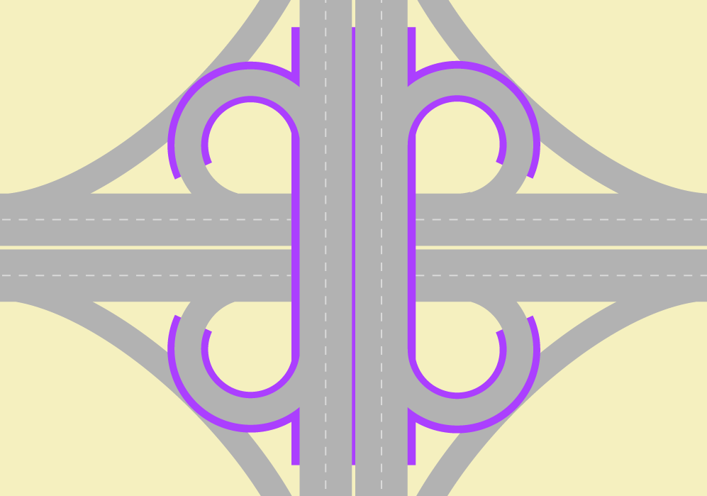
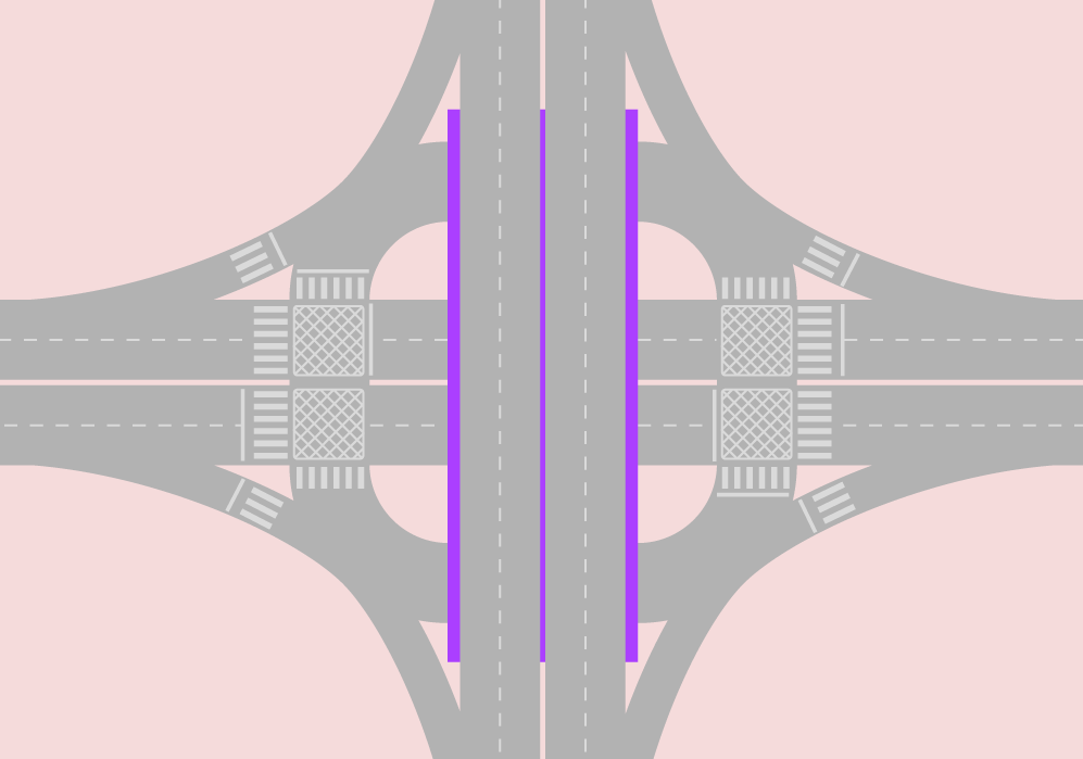
In theory, a separated-grade traffic solution eliminates intersections (Figure 24.3), but in practice, due to space restrictions, intersections can also remain (Figure 24.4).
24.1.2General Concepts
The concepts we present here are mostly about understanding the equations related to delay and queue sizes in signalized intersections, but note that these sections are not meant to be a comprehensive reference for these issues. The reader may want to further investigate the concepts of traffic density and traffic headway and how they relate to average traffic speed and flow. We provide further references for traffic signals in the bibliography.
We emphasize that when applying formulas attention should be given to units and unit conversions. The appropriate unit of time to observe phase times in traffic lights is the second, which can be used to observe the time to walk or ride a few blocks; meanwhile, we better perceive speeds in kilometers per hour (kph) or alternatively in miles per hour (mph). It is useful to remember that 1 hour is the same as 3,600 seconds and 1 mile is approximately 1.6 kilometers and 1 kilometer is approximately 0.6 miles.
24.1.2.1Cross-Traffic Turn and Curbside Turn
For this chapter we have excluded the expressions “right turn” and “left turn” because they have different meanings in differently oriented systems. We have chosen to adopt “cross-traffic turn” and “curbside turn” instead.
Cross-Traffic Turn: a vehicle movement to exit the current traffic stream direction that requires crossing the opposite-direction traffic flow. If a busway or a bike lane is present near the median, there is also conflict with BRT vehicles or bicycles going straight in the same way and in the opposite way.
Curbside Turn: a vehicle movement to exit the current traffic stream direction that normally does not cross any vehicle flow. This movement conflicts with people on the sidewalk in both ways and, if the road is parallel to a curbside busway or a curbside bike lane, there is a conflict with that traffic as well.
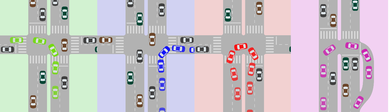
U-Turn: a vehicle movement to join the traffic stream travelling in the opposite direction of the vehicle’s current flow. Depending on the width of the median this movement can be less conflicting than the cross-traffic turn or more conflicting, since the speed has to be lower to make a U-turn. For this reason, U-turns are sometimes prohibited at existing intersections and promoted away from the intersection by creating another intersection exclusively for the U-turn. Due to road geometry restrictions or other considerations, this movement may eventually be channeled to start from a waiting area from the curb side of the road as shown by the pink car in Figure 24.5, in which case it will conflict with both flows in the same way that a cross-traffic turn from a perpendicular street would.
24.1.2.2Speed
For the application of the concepts outlined in this chapter, speed is defined as the average traffic speed of all vehicles in a segment, for which we use the letter V that is derived from the word velocity. Speed is measured by the mean time of all vehicles crossing the segment divided by the segment extension. Under our modeling intents (or capacity evaluation) it can be imagined that all vehicles are moving at that speed.
Still, when looking at the broader concept of speed—the ratio of motion expressed in distance per unit of time—it is useful to remember that for a given segment distance (Dsegment), knowing the speed (Vsegment) is equivalent to knowing the travel time it takes to make it through the segment (Timesegment) and vice versa, as the equivalent equations show:
Eq. 24.1
\[ V_\text{segment} = {D_\text{segment} \over \text{Time}_\text{segment}} \leftrightarrow \text{Time}_\text{segment} = {D_\text{segment} \over V_\text{segment}} \]
Where:
- \( V_\text{segment}\): Velocity of the segment;
- \( D_\text{segment}\): Segment distance;
- \( \text{Time}_\text{segment} \): Travel time it takes to make it through the segment.
24.1.2.3Delay
Delay is the additional travel time, if not explicit, that is added onto the base reference of travel time, which is an ideal situation without any conflicts where the passenger, pedestrian, or driver is the only user of the road (no other drivers, pedestrians, users, or traffic lights).
24.1.2.4Passenger Car Unit (pcu)
A passenger car unit, or pcu, is a reference used to standardize different vehicle types by a common denominator. The conversion factor from a certain type of vehicle to a passenger car unit depends on the application intended after the conversion, when it is eventually calibrated for a specific use in a given situation. For example, this could be when consideration is given to the stress placed on the pavement or the potential of added congestion. Other considerations include whether the setting is an urban environment or along a highway, on a ramp, or in plain terrain.
In general, a motorcycle, for instance, tends to have an equivalent of less than one vehicle, and a mini-bus is equivalent to more than one vehicle; the larger and heavier the vehicle, the higher the number of vehicles to which it is equivalent.
24.1.2.5Flow
Traffic engineering borrows concepts from fluid mechanics and uses “flow rate” as a measure of traffic intensity. From that definition, the word rate is commonly dropped and “flow” alone is treated as the physical quantity expressed by the number of vehicles crossing a transversal section (or cross section, like a stop line) during a certain time interval. Flow is usually represented by the letter q in equations, but we will avoid that here and use the full word instead.
It should be noted that the use of the word volume to express the same idea is accepted, despite being far from the original definition conceptually (in fluid mechanics the original comparative terms are volume flow rate and mass flow rate; the latter is more an appropriated reference as the vehicles can be somewhat compressed). Volume should refer to the total number of vehicles in the same way a liter refers to volume and liters per second refers to flow in hydraulics. The term is especially common in the expression “volume/capacity ratio.”
Eq. 24.2
\[ \text{Flow}_\text{vehicles} = {Number_\text{vehicles} \over \text{Time}} \]
Where:
- \( \text{Flow}_\text{vehicles} \): Number of vehicles crossing a transversal section (or cross section, like a stop line) per a given time;
- \( \text{Number}_\text{vehicles} \):Number of vehicles;Time = Length of time the flow of vehicles is measured.
Flow can also be expressed for pedestrians, bicycles, or even passengers (per hour).
24.1.2.6Capacity and Saturation
The capacity (flow rate) of a segment is given by the lower capacity of a section within it, and the term bottleneck for the lower-capacity section expresses this concept quite well.
The capacity of a section is defined as the maximum flow a section can handle under prevailing use. It is subject to the number of lanes, width of lanes, ramp inclination, cultural driving behaviors, and the use of surrounding areas, such as parking and stopping regulations, the presence of an intersection or traffic light ahead, and the existence and frequencies of bus stops.
Capacity can easily and objectively be measured, but some of the influential factors listed above cannot. Many models have been developed to improve the forecast of road capacity based on the knowledge of design and use of surroundings, but even the more detailed simulators need careful calibration to correctly represent driver behavior differences that tend to be unique to each place.
The simpler models do not commonly fit exactly to theories, either, and they are usually adjusted by experimental evidence. These models resort to the concept of basic saturation flow.
Basic saturation (flow rate) is the capacity for a section of a given standard ideal roadway, divided by the number of lanes of that given standard roadway. It is commonly expressed by “s0.”
Capacity and speed are interdependent and the maximum flow does not happen when speeds are at their highest. This is because the distance a driver maintains from another vehicle in front of him or her increases more proportionally than the speed increases. In a section of unconstrained road, the maximum speed capacity occurs between 60 and 80 kilometers per hour.
Based on extensive observations, capacity models then define a way to forecast a saturation flow by multiplying the basic saturation flow by adjustment factors to account for various nonideal geometric, traffic, and environmental conditions of a given section, such as the number of lanes, lane width, presence of heavy vehicles, grade, parking facilities, bus blockage, area type, turning traffic along the segment, radius of turnings, pedestrian crossing traffic, but not considering traffic lights.
Saturation is commonly written as “S” in equations, but here we use “SaturationFlow” to avoid confusion with demand saturation level, usually “X,” which represents the relationship between demand and capacity for a given infrastructure element such as an intersection or a station.
Eq. 24.3
\[ \text{Saturation}_\text{Flow} = \text{basicsaturationflowperlane}*NLanes*(f_\text{geometry}*f_\text{traffic}*f_\text{parking} * f \ldots) \]
Where:
- \( \text{SaturationFlow} \):Maximum flow a section can handle under prevailing use;
- \( \text{basicsaturationflowperlane} \): Capacity of a given standard ideal roadway section;
- \( \text{NLanes} \): Number of lanes;
- \( f_\text{geometry} \): Adjustment factor to account for nonideal geometric conditions;
- \( f_\text{traffic} \): Adjustment factor accounting for nonideal traffic conditions;
- \( f_\text{parking} \): Adjustment factors to account for nonideal parking conditions;
- \( f\ldots \): Other adjustment factors to account for various nonideal conditions.
Saturation (flow rate), therefore, is the capacity of a section that is not under the influence of a traffic light. For a section that approaches a traffic light, saturation is the capacity assuming a constant green, which would equal the flow observed during the queueing discharge (after allowing a few seconds for the flow to become regular again). For this reason saturation may be called discharge (flow rate). When working in a specific location, the saturation of sections can be measured, so the resulting product of all these factors is known.
As a practical rule, even slightly distorting the concept of ideal conditions for urban environments will yield an observed saturation of 1,800 pcu/hour for a lane. For the purpose of capacity, measuring an 18-meter articulated bus is equivalent to 2.5 pcu. So in a busway the saturation per lane is 720 articulated buses per hour.
Eq. 24.4
\[ \text{SaturationFlow}=\text{CapFlow}_\text{away-from-intersectioni} = \text{saturationflowperlane} * \text{NLanes} \]
Where:
- \( \text{SaturationFlow} \): Maximum flow a section can handle under prevailing use;
- \( \text{CapFlow}_\text{away-from-intersection} \): Maximum flow of a section away from an intersection;
- \( \text{saturationflowperlane} \): Maximum flow a given lane can handle;
- \( \text{NLanes} \): Number of lanes.
24.1.2.7Continuity
Although no direct formula application about continuity is used in this chapter, one basic property of an intersection is that all the flow into the intersection has to exit the intersection.
24.1.3Traffic Signal Concepts
Traffic lights are a very common intersection management tool in business districts where the BRT corridor design is likely to face more challenges. Traffic light controllers can be coordinated and actuated (use detection) by utilizing more or less complex technology and algorithms. A lot of research and progress has been made in the past thirty years, but the practical use of the research is still relatively limited. The concepts presented in this chapter are helpful in understanding BRT design requirements to program traffic lights, be it on simple controllers or as policy delimiters to more complex systems.
Traffic lights eliminate some of the negotiations between vehicles on arrival by determining which movements may proceed at a given moment. Traffic lights may allow conflicting movements, usually not all of them are intense; pedestrians crossing the transversal street are a common one. By reducing negotiations, traffic lights prevent vehicles approaching the intersection from reducing their speeds, raising the time each vehicle spends in the intersection itself (which, by definition, is an area). Traffic signals increase the throughput while keeping intersections safe.
24.1.3.1Phase
One set of movements that is allowed to occur at the same time is called a signal phase. It should be noted that some movements are allowed during several phases; in many countries, allowing curbside turns at all times is the standard. Some may use expressions like “allowing a particular turn in the beginning of phase two” when technically it should be “adding a short phase before phase two where a particular turn will be allowed.”
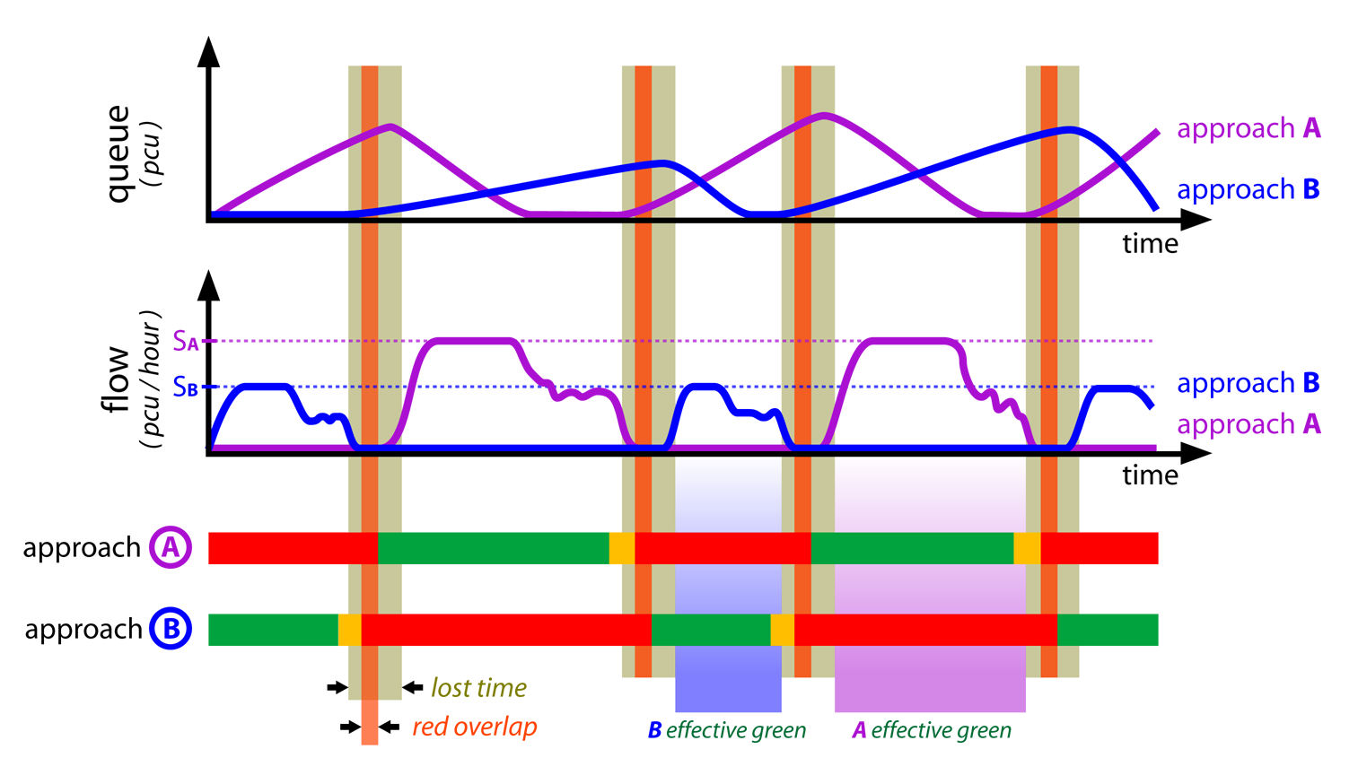
24.1.3.2Effective Green Time (Tgreen)
The phase duration (or length) refers to its “effective green time,” which is the time vehicles are considered effectively moving, which may start a little after the green light is given and end in the middle of yellow lights (where such are used), or in the first moments of red (clearance interval). For this chapter, where queueing and intersection capacity are evaluated, green time means “effective green time.”
24.1.3.3Cycle Time (Tcycle)
Excluding situations where special phases are activated by detectors, the traffic signals in an intersection repeat the order of the phases successively in cycles. The cycle time can be measured as the time between when the green light is given until the next time it is given again (after it has changed to red once). In this chapter, “cycle time” alone refers to a traffic light cycle time (route cycle times are not discussed).
24.1.3.4Red Time (Tred)
For the interest of intersection capacity and queueing evaluation, red time means cycle time minus (effective) green time.
24.1.3.5Lost Time
Lost time is the period between the end of the effective green of a phase and the start of the next. Lost time depends on the signal programming for yellow times and overlapping red (clearance red). It also depends on the enforcement policy and driver behavior (longer lost times are associated with safer intersections), but for the given conditions, there are fixed values.
We refer to lost time as the total lost time per cycle, but lost time can be further split into the start-up and clearance for each phase, each of them being nearly two seconds. One can generally consider that a four-phase signalized intersection has lost a time of sixteen seconds, meaning that the total lost time each cycle is sixteen seconds.
24.1.3.6Traffic Light Plans
In the same way for intersections in general, the higher the number of turning movements there are in an intersection with traffic lights, the more difficult it is to serve them all. Some movements can happen simultaneously, while some cannot. Reducing the number of phases implies that the number of lanes allowing movements on any phase will be higher, and it also implies that the intersection will have a higher overall throughput (see Section 24.5: Restricting General Traffic Movements).
The optimal phase times in a signalized intersection are such that the cycle time is as brief as possible without growing queues. Having the minimum cycle is optimal because it implies the shortest possible red times, which is similar to the shortest possible waiting times. In order to not have queues, if demand and saturation flow is known for each approach, the minimal number of effective green seconds per hour required can be calculated for an approach that does not form queues. If this is calculated for all approaches, the minimum effective green time for that intersection as a whole is known, and the total number of effective green seconds in an hour shall be way below 3,600, leaving the difference to be designated as lost time.
Contradictory as it seems at first, the best signal programming is such that it has the maximum lost time per hour, because that implies the highest number of cycles per hour. For example, if required green time for vehicles in the intersection is 3,200 seconds, the intersection is close to collapsing. This is because there are only 400 seconds per hour to allow pedestrian crossings and lost time still needs to be added. Assuming there are two vehicle phases plus a minimal pedestrian phase of 6 seconds, and an extra 4 seconds for each phase change, each cycle will need an additional 18 seconds (= 6 + 4 * 3) beyond vehicle green time. This extra time for all cycles during one hour is defined as 400 seconds, so the intersection can have a maximum of 22 complete cycles (= 400 / 18) or 162 seconds (almost 3 minutes) of cycle time.
Time of day should be taken into consideration because infrastructure that is sized based on the peak use may eventually become underused at other times of the day. Traffic signal timing plans for peak moments could lead to unnecessary delays at other points during the day. Traffic light plans should change throughout the day as demand changes; one extreme example of this is shutting down a signal during late night and early morning hours (or switching to a yellow blinking signal).
Traffic signal programming shall change throughout the day, so that green and red cycle times must change based on different programming for the time of the day (as well as week and season) and, where available, change based on traffic detection applied to parameters in the programming for that moment. When we discuss these features as fixed, we must understand them as the limiting parameters for the traffic controller that allow adaptive changes based on detection.
We look at infrastructure layouts associated with the traffic-signal plan for the peak hours of the day for each flow, and if there is enough capacity during this time frame, then there certainly will be in others, although traffic signal programs need to be different to minimize travel times. To represent the peak, we use and measure the busiest hour of the day for the given flow (as a reminder: we survey data with smaller intervals than one hour, so a given measure of the busiest hour might have happened from 7:15 a.m. to 8:15 a.m., for example).
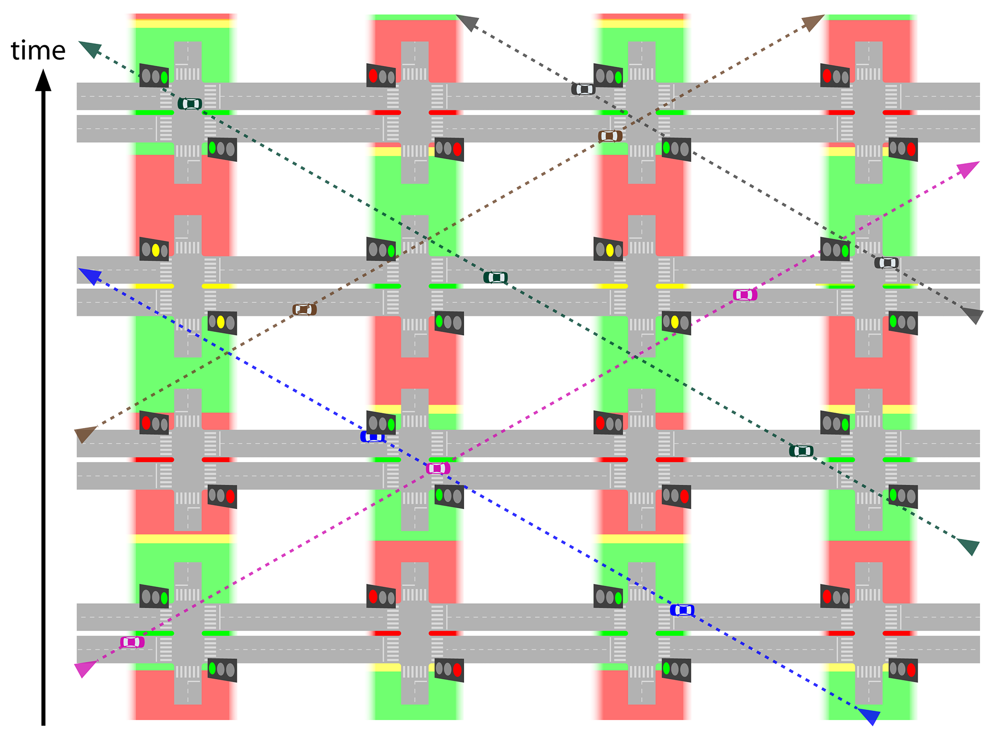
24.1.3.7Traffic Signal Coordination
Coordination is the synchronization of several traffic lights along a path to produce a “green wave” for that route, eliminating waiting while still keeping the required/projected capacity for all flows. With proper planning, it is possible to coordinate several routes (including pedestrians and to some extent, public transport) in the same area by establishing priorities among them. Eventually, routes with lower priority end up having more breaks in their green waves and some intersections will need to have irregular green times for the transversal flows (still fixed in a larger cycle measure: one long, one short, one long, one short, and so on).
24.1.3.8Detection or Actuation
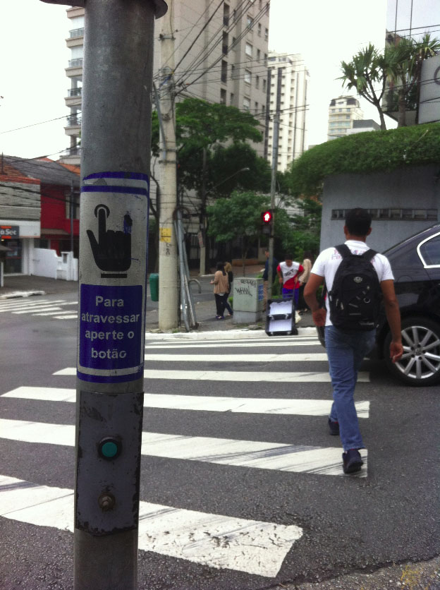
Actuation is the form in which the user informs his or her presence to a traffic signal controller, for example:
- A pedestrian pressing a button to request a crossing (Figure 24.9);
- A vehicle passing over a magnetic induction loop buried in the traffic lane (Figure 24.10).
Actuation can be used in many ways, isolated or in conjunction with traffic control signs:
- Add a required phase for pedestrians or cross-traffic turns (semi-actuated control);
- Determine the length of every phase (full-actuated control);
- Activate a preestablished plan that will eventually be coordinated (actuated pre-time control);
- Establish public transport priority (see Section 24.3.2: Active Signal Priority);
- Input data about movement requests to a central traffic control that computes several inputs at once to select a plan of operation;
- Input data about movement requests to central controllers that adjust traffic signal parameters by evaluating alternative strategies for the requirements in real time (adaptive control, among which “Split Cycle Offset Optimization Technique” or “SCOOT model” is a common reference for this type of adaptive central controller).
24.1.3.9Intersection Capacity
Considering the definition of an intersection as the area where vehicles come into conflict, the capacity of the intersection should be measured as the total number of (equivalent) vehicles that cross it, tallying the total of all the movement.
But for the purposes of this chapter, intersection capacity refers to the entrance section (the approach or stop line) of only the road segment being analyzed. Furthermore, we are particularly interested in signalized intersections, assuming that the corridor where the BRT is placed has preference at smaller non-signalized intersections that do not cause other meaningful interference to mixed traffic or to BRT, which is not included in the basic saturation flow measures.
24.1.3.10Relative Green (Kgreen)
The proportion of time allowed by a green light for a flow to cross an intersection (Kgreen) is given by the equation below.
Eq. 24.5
\[ K_\text{green} = {T_\text{green} \over T_{cycle} }\]
Where:
- \( K_\text{green} \): Relative green, or the proportion of time given by a green light for a flow to cross an intersection;
- \( T_\text{green} \): Time given by a green light for a flow to cross an intersection;
- \( T_\text{cycle} \): Time given by the signal cycle.
The previous and following equations apply to fixed cycles, but to measure the relative green of a coordinated traffic light with irregular times, one should consider the total green time along a repetition cycle (short, long).
24.1.3.11Relative Red (Kred)
The proportion of time that traffic is held by a red light in a given approach (Kred) is given by the equation below.
Eq. 24.6
\[ K_\text{red} = {T_\text{red} \over T_{cycle}} \]
Where:
- \( K_\text{red} \): Relative red, or the proportion of time that traffic is held by a red light in a given approach;
- \( T_\text{red} \): Time given by a red light holding traffic from crossing an intersection;
- \( T_\text{cycle} \): Time given by the signal cycle.
By the relation of this definition and that of red time, \( T_\text{red} = T_\text{cycle} - T_\text{green} \), we can conclude that \( T_\text{red} + T_\text{green} = T_\text{cycle} \leftrightarrow {T_\text{red} \over T_{cycle}} + {T_\text{green} \over T_{cycle} } ={T_\text{cycle} \over T_{cycle} } \leftrightarrow K_\text{red} + K_\text{green} = 1 \) and therefore:
Eq. 24.7
\[ K_\text{red} = 1 - K_\text{green} \]
Where:
- \( K_\text{red} \): Relative red, or the proportion of time that traffic is held by a red light in a given approach;
- \( K_\text{green} \): Relative green, or the proportion of time given by a green light for a flow to cross an intersection.
Eq. 24.8
\[ K_\text{green} = 1 - K_\text{red} \]
Where:
- \( K_\text{red} \): Relative red, or the proportion of time that traffic is held by a red light in a given approach;
- \( K_\text{green} \): Relative green, or the proportion of time given by a green light for a flow to cross an intersection.
24.1.3.12Capacity at a Signalized Intersection Approach
The capacity at a signalized intersection approach is simply the saturation flow of the approach multiplied by the proportion of time it is in operation. Unless stated otherwise, intersection capacity refers to this.
Eq. 24.9
\[ \text{CapFlow}_\text{intersection} = \text{saturationflowperlane} * \text{NLanes} * K_\text{green} \]
Where:
- \( \text{CapFlow}_\text{intersection} \): Capacity at a signalized intersection approach;
- \( \text{saturationflowperlane} \): Maximum flow a given lane can handle;
- \( \text{NLanes} \): Number of lanes;
- \( K_\text{green} \): Relative green, or the proportion of time given by a green light for a flow to cross an intersection;
The capacity away from the intersection can be considered by this definition, if one assumes that \(K_\text{green}\) is equal to one—that is, an uninterrupted flow.
Eq. 24.10
\[ \text{CapFlow}_\text{intersection} = \text{saturationflowperlane} *NLanes \]
Where:
- \( \text{CapFlow}_\text{intersection} \):Capacity at a signalized intersection approach;
- \( \text{saturationflowperlane} \): Maximum flow a given lane can handle;
- \( \text{NLanes} \): Number of lanes.
24.1.3.13Demand Saturation Level (X)
Demand saturation level is a dimensionless form of expressing demand by comparing it to the maximum that the infrastructure under analysis can serve. Applied to a road section, it is given by demand flow (how many vehicles want to cross the section for the duration of time interval) over the saturation flow. This means that if the section is the entrance to an intersection, the reference is the discharge flow rate (how many vehicles can cross the section if the traffic light is green during the whole interval).
Eq. 24.11
\[ X = {\text{DemandFlow} \over \text{SaturationFlow}} \]
Where:
- \( X \): Demand saturation level;
- \( \text{DemandFlow} \): Number of vehicles that want to use the section for the time interval;
- \( \text{SaturationFlow} \): Maximum flow the section can handle under prevailing use;
Demand saturation level is sometimes referred to as “saturation level” or just “saturation,” which can create confusion with “saturation flow.” Also, we use “demand level” and “X” in this chapter.
24.1.3.14Demand to Signal Capacity Level (XSignal)
This is a variant form of expressing demand saturation level at the traffic light, and instead of comparing it to the maximum possible throughput, this compares it with the possible throughput under current programming. It is given by demand flow over capacity flow. The reference is the traffic sign effective capacity (how many vehicles can cross the section during the interval that the traffic light is green).
Eq. 24.12
\[ \text{XSignal} = { \text{DemandFlow} \over \text{CapacityFlow}} \]
Where:
- \( \text{XSignal} \): Demand to signal capacity level;
- \( \text{DemandFlow} \): Number of vehicles that want to use the section for the time interval;
- \( \text{CapacityFlow} \): Maximum flow that can cross the section during the interval that the traffic light is green.
Eq. 24.13
\[ \text{XSignal} = { \text{DemandFlow} \over \text{SaturationFlow} * K_\text{green} } \]
Where:
- \( \text{XSignal} \): Demand to signal capacity level;
- \( \text{DemandFlow} \): Number of vehicles that want to use the section for the time interval;
- \( \text{SaturationFlow} \): Maximum flow a section can handle under prevailing use;
- \( K_\text{green} \): Relative green, or the proportion of time given by a green light for a flow to cross an intersection.
Demand to signal capacity level is particularly relevant for the calculation of traffic sign delay below in the particular formulation we use. Sometimes it is called “signal saturation level” as the following definition is also possible.
Eq. 24.14
\[ \text{XSignal} = {X \over K_\text{green} } \]
Where:
- \( \text{XSignal} \): Demand to signal capacity level;
- \( X \): Demand saturation level;
- \( K_\text{green} \): Relative green, or the proportion of time given by a green light for a flow to cross an intersection.
Signal Delay (\(T_\text{signal}\))
The calculation assumes that arrivals are random and departure headways are uniform, which is applicable only for undersaturated conditions and predicts infinite delay when arrival flows approach capacity. This is realistic for design purposes, as we intend to promote undersaturated conditions.
Signal delay is composed of two terms:
- The first term (\(T_\text{queue}\)) is the delay due to a uniform rate of vehicle arrivals and departures at the signal;
- The second term (\( T_\text{random}\)) is the random delay term, which accounts for the effect of random arrivals. But if demand of signal capacity level is below 50 percent, then it should be ignored.
Eq. 24.15
\[ T_\text{signal}=T_\text{queue}+T_\text{random} \]
Where:
- \( T_\text{signal} \): Signal delay;
- \( T_\text{queue} \): Delay due to a uniform rate of vehicle arrivals and departures at the signal;
- \( T_\text{random} \): Random delay term, which accounts for the effect of random arrivals.
The first term is deductible as the area below the queueing in Figure 24.7 over the number of vehicles during a cycle (\( \text{DemandFlow} * T_\text{cycle}\)).
Eq. 24.16
\[ T_\text{queue}={ T_\text{red}^2 \over 2 * T_\text{cycle} * (1-X)} \]
Where:
- \( T_\text{queue} \): Delay due to a uniform rate of vehicle arrivals and departures at the signal;
- \( T_\text{red} \): Time given by a red light holding traffic from crossing an intersection;
- \( T_\text{cycle} \): Time given by the signal cycle.
The extra delay in queuing, caused by the non-regularity of arrivals in the traffic light (\(T_\text{random}\)) is a function of the demand-to-signal capacity level (\(\text{XSignal}\)) and a regularity of vehicles (buses in our case) arrival coefficient (\(K_\text{reg}\)).
If the signal saturation (\(\text{XSignal}\)) is low, the randomness of arrivals will not generate extra time in queueing formation. As the signal saturation increases, the impact on extra time due to the expected randomness of arrivals becomes bigger than the increments. If the signal saturation is bigger than one (there are more vehicles willing to use the lane than what the traffic light can handle), there will be severe busway congestion (congestion would happen even if there were no random arrivals at all). So, the extra queueing delay due to randomness is calculated by:
Eq. 24.17
If \( \text{Xsignal} < K_\text{reg} \), then \( T_\text{random} = 0 \)
If \(K_\text{reg} \leq \text{Xsignal} < 1\), then: \( T_\text{random} = {{\text{XSignal} - K_\text{reg} \over 1 - \text{XSignal} } * 1 \over \text{SaturationFlow}} \);
If \( \text{Xsignal} \geq 1 \), then there would be severe congestion (\(T_\text{random} \to \infty \)).
Where:
- \( \text{XSignal} \): Demand to signal capacity level;
- \( \text{Trandom} \): Random delay term, which accounts for the effect of random arrivals.
- \( \text{SaturationFlow} \): Maximum flow a section can handle under prevailing use;
\( K_\text{reg} \): Regularity factor; it is a number related to the chance a bus has to arrive within the signal cycle as detailed below:
- It would equal one if there were total regularity in vehicle arrivals;
- It would be 0.5 if half of the vehicles arrive more than one signal cycle later than when they are expected;
- The value used to represent uncertain arrivals is 0.5.
This formula is a variation of the model proposed by Webster in 1958, slightly simpler than originally proposed but with a smoother transition when the random delay becomes more relevant than the practical modification most commonly applied.