24.4Station Location Relative to the Intersection

24.4.1Station Location Possibilities

The following station locations are possible:

• At the intersection:

  • For side-aligned stations, the station can be either nearside or far side—that is, before or after the intersection in each direction;
  • For median stations, if not split, the station will be nearside in one direction and far side in the other;

• Away from the intersection;

  • Near the intersection;
  • Far from the intersection (or mid-block);
• Under or over the intersection.

24.4.1.1At Intersections

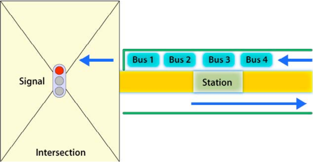
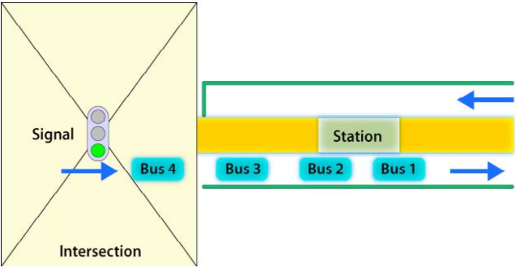
The normal justification for putting the bus stop at the intersection is that it reduces walking times for customers with destinations or transferring on the crossing street. Unless the red time is really short (fewer than twenty seconds) and station saturation (discussed in Chapter 7: Capacity and Speed) is really low, the resulting saturation of the combination of the intersection plus station (i.e., the proportion of time a BRT vehicle will occupy the area with two functions: queue-box waiting for green light and boarding area) is likely to be greater than one, and this will lead to congestion that will end only after the peak (Figure 24.20). Such a situation clearly will not be compensated for by reducing customer walking times. It also will not be of help to customers that are alighting at that station or must only cross that intersection.

Additionally, such justification is often based on presumptions and rarely on data; only micro-level destination maps based on surveys can effectively quantify walking time benefits of station location relative to the intersection. Furthermore, the large number of transferring customers should be prevented when route service planning is designed.

In the rare case that the station must be located at the intersection, there is an emerging consensus that locating the station before the intersection is preferable, particularly in split platform configurations if the BRT lane is near the median.

24.4.1.2Away from the Intersection

Stations should in general be around a hundred meters from intersections. As highlighted above and as discussed in the remainder of this section, there should be some space between the intersection and the station since it:

• Provides the possibility of taking away mixed-traffic space without changing road capacity for the section;
• Prevents bus queues at the intersection from hindering the station;
• Leaves width at the intersection for increasing mixed-traffic capacity and turns (Figure 24.21).

We further divide the description of the station’s location into “near it” or “far from it” (or "mid-block") with regard to the intersection. The aspect to be taken into consideration here is customer access to the station.

Mid-block stations will require access infrastructure not shared nor closely related to the intersection’s pedestrian crossings. In the typical environment discussed here, that is, a station located between mixed-traffic signalized intersections, signalized at-grade options are the likely ideal solutions. But such a solution introduces a new intersection (considering the multimodal definition of it) that needs to be taken into account when evaluating capacity of both the station and mixed-traffic.

We should remember that a crossing for access will be required for curbside mid-block stations as well. Mid-block stations are arguably safer to access than near-intersection stations and cycle times can be shorter. Saturation correction must be applied (see Section 24.4.6: Correction Factor for Station Saturation at Traffic Light).

24.4.2Minimizing the Number of Mixed-Traffic Lanes Away from the Intersection

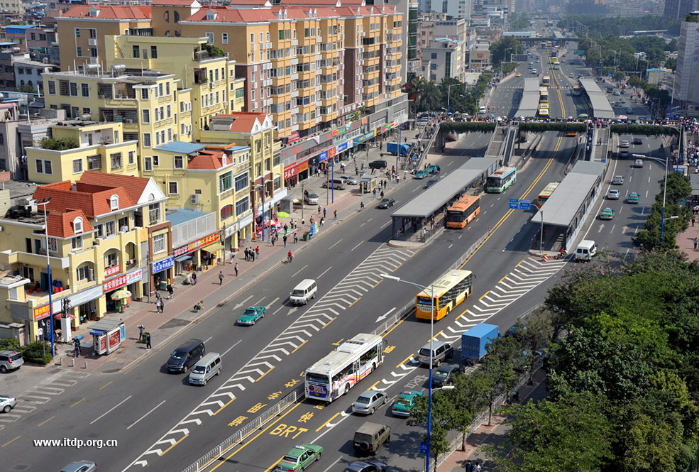
Usually the mixed-traffic bottleneck is the intersection, where capacity is 50 to 30 percent (proportional to the green fraction of each approach) of mid-block capacity. So if BRT stations are far from intersections, the general-traffic road capacity can be reduced in its surroundings without any significant impact on the capacity and performance on the segment as a whole. This means that mixed-traffic lanes can be removed, and the space given to the BRT station, thus enabling the widening required for BRT at stations to accommodate passing lanes, and hence provide high capacity at stations without impacting mixed-traffic capacity at all (Figure 24.23).

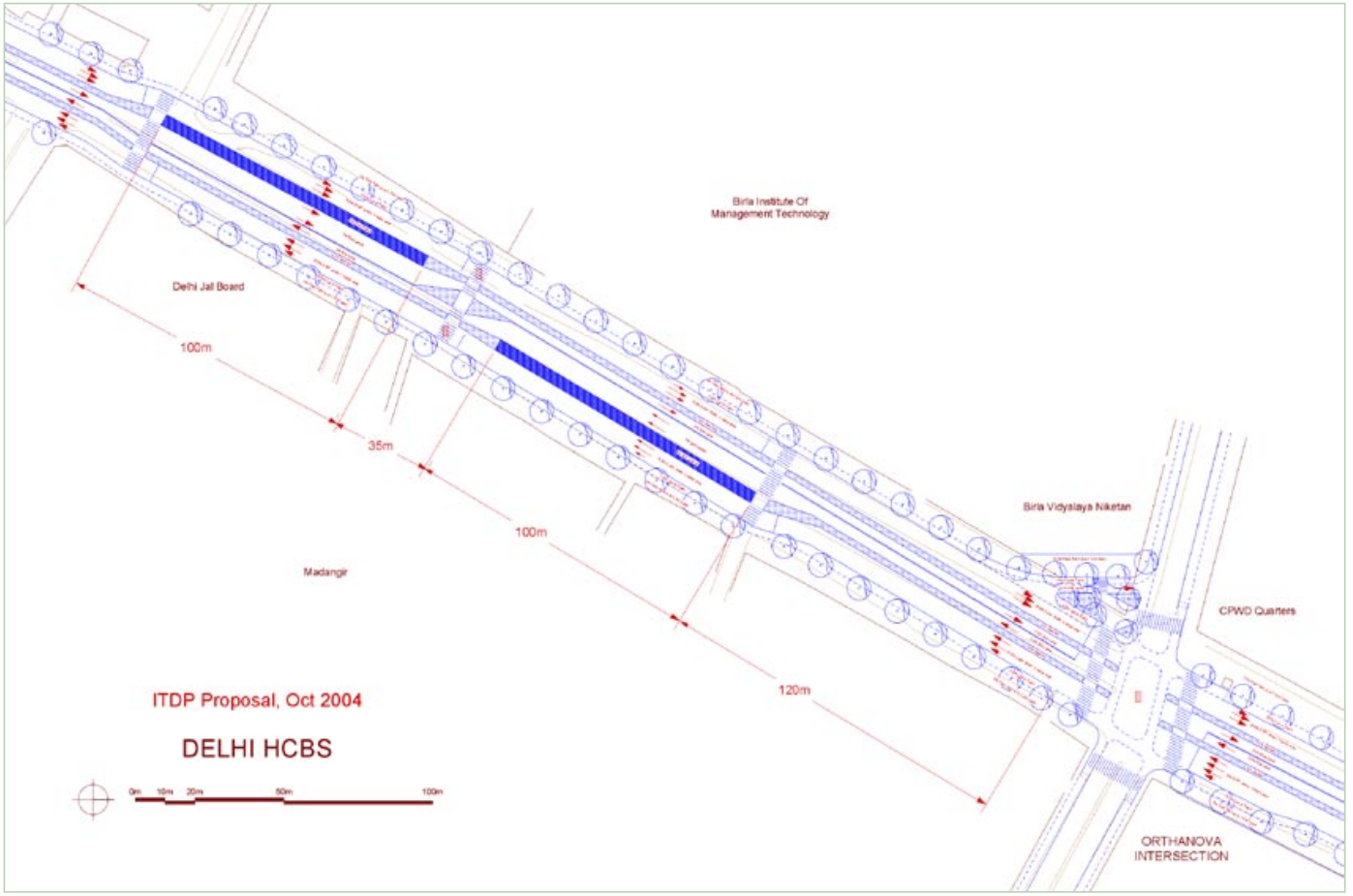
For example, at the bus stop, if bus frequencies are high and an overtaking lane is needed at each station, the extra width required will be around 12 meters. If the station is located at the intersection, these 12 meters will be difficult to supply while also providing 6-meter turn lanes for mixed traffic. Separating these functions will allow the same right-of-way to be used for the bus station at mid-block, and for left and right turn signals at the intersection. Figure 24.22 shows an application of this concept within a proposal for the Delhi BRT system.

Capacity in a given control section (CapFlow) is expressed in the equation below.

Eq. 24.18

\[ \text{CapFlow}_\text{intersection} = \text{saturationflowperlane} * \text{Nlanes} * K_\text{green} \]

Where:

• \( \text{CapFlow}_\text{intersection} \): Capacity of the evaluated section of control, usually in pcu/hour;
• \( \text{saturationflowperlane} \): Saturation flow of one lane (in “ideal conditions,” around 1,800 in urban areas pcu/hour);
• \( N_\text{lanes} \): Total number of available lanes;
• \( K_\text{green} \): Relative (effective) green time, which is given by Equation 24.5:

\[ K_\text{green} = { T_\text{green} \over _\text{Tcycle} }\]

Where:

• \( K_\text{green} \): Relative green, or the proportion of time given by a green light for a flow to cross an intersection;
• \( T_\text{green} \): Time given by a green light for a flow to cross an intersection;
• \( T_\text{cycle} \): Time given by the signal cycle.

One can evaluate the possibility of narrowing the mixed-traffic road away from the intersection without affecting the capacity of the segment by assuring that capacity away from the intersection (where relative green time can be considered 1 or 100 percent) is greater than capacity in the intersection.

\[ \text{FlowCap}_\text{away} \geq \text{FlowCap}_\text{intersection} \]

\[ \text{saturationflowperlane} * \text{NLanes}_\text{away} * K_\text{green away} \geq \text{saturationflowperlane} * \text{NLanes}_\text{intersection} * K_\text{green intersection} \]

\[ \text{NLanes}_\text{away} * K_\text{green away} \geq \text{NLanes}_\text{intersection} * K_\text{green intersection} \]

\[ \text{NLanesaway} \geq \text{NLanes}_\text{intersection} * {K_\text{green intersection} \over K_\text{green away}} \]

Examples:

• If near-intersection mixed traffic has 3 lanes (\(\text{NLanes}_\text{away} = 3\)), and relative green time is 60 percent (\( T_\text{green} \over T_\text{cycle} = 0.6 \)), then far from intersection (\(\text{Nlanes}_\text{away}\)) can be 2 lanes without affecting the segment performance:\( \text{NLanes}_\text{away} \geq 3 * 0.6 = 1.8 \) ;
• If near-intersection mixed traffic has 2 lanes (\(\text{NLanes}_\text{away} = 2\)), and relative green time is 50 percent (\( T_\text{green} \over T_\text{cycle} = 0.5 \)), then far from intersection (\(\text{Nlanes}_\text{away}\)) can be only one lane without affecting the segment performance: \( \text{NLanes}_\text{away} \geq 2 * 0.5 = 1.0 \) ;
• If we are planning a mid-block station with signalized pedestrian crossing for the first example, we would have to keep relative green for traffic mid-block above 90 percent.

24.4.3Minimizing the Recommended Distance between the BRT Station and the Intersection from a Mixed Traffic Perspective

NOTE: THIS DISTANCE IS FOR STATIONS THAT TAKE AWAY MIXED-TRAFFIC LANES, NARROWING THE AVAILABLE SPACE FOR CARS AWAY FROM THE INTERSECTION AND ENSURING THAT MIXED-TRAFFIC CAPACITY IS NOT AFFECTED!

Away from the signalized intersection means far enough to guarantee that the capacity flow in the intersection can last the entire green phase. This is equivalent to ensuring that the queueing space with the same number of lanes of the intersection approach has enough capacity to hold all vehicles that can cross the intersection in the duration of the green phase.

This means the distance from the intersection (Diststation-intersection) has to be greater than the space for queueing vehicles times the number of vehicles that will cross the retention line in one lane.

Considering a saturation flow per lane (saturationflowperlane) of 1,800 pcu/hour is equivalent to one vehicle every two seconds (passing across the intersection in one lane) and the distance between (the front of) two vehicles (lengthpcu) is 5 meters, this implies that for each second of the green phase the queue will be 2.5 meters short.

\[\text{Queue discharge rate} = {\text{flow}_\text{saturation} \over \text{length}_\text{pcu}} \]

Another way to think about this is that the “speed of the shock wave” starting at the retention line after the traffic signal opens is 2.5 meters per second. That is, the second car behind (5 meters behind) will start to move 2 seconds after the first, the third car behind (10 meters from the retention line) will move after 4 seconds and so on.

\[\text{Velocity}_\text{discharge shockwave} = {\text{flow}_\text{saturation} \over \text{length}_\text{pcu}} \]

Therefore the distance between station and intersection (Diststation-intersection) has to be equal to or greater than the distance that the shock wave can move during the duration of the green phase (Tgreen). Representing the speed of shock wave by Velshock-wave, this can be expressed as:

\[ \text{Dist}_\text{station intersection} \geq V_\text{shock wave} *T_\text{green}\]

Using meters and seconds for the measures we have:

Eq. 24.19

\[ \text{Dist}_\text{station intersection} [\text{in meters}] \geq 2.5 * T_\text{green} [\text{in seconds}] \]

Where:

• \( \text{Dist}_\text{station-intersection} \):Distance between station and intersection;
• \( T_\text{green} \): Time given by a green light for a flow to cross an intersection.

Examples:

• If green time is 40 seconds, the station must be at least 100 meters from the intersection, equal the length of queue discharged during the green time:

\[ \text{Dist}_\text{station-intersection} [\text{in meters}] \geq 2.5 * 40 = 100 \]

• If green time is 90 seconds, the station must be at least 225 meters from the intersection, equal the length of queue discharged during the green time:

\[ \text{Dist}_\text{station-intersection} [\text{in meters}] \geq 2.5 * 90 = 225 \]

24.4.4Minimizing the Recommended Distance between the BRT Station and the Intersection from a BRT Perspective

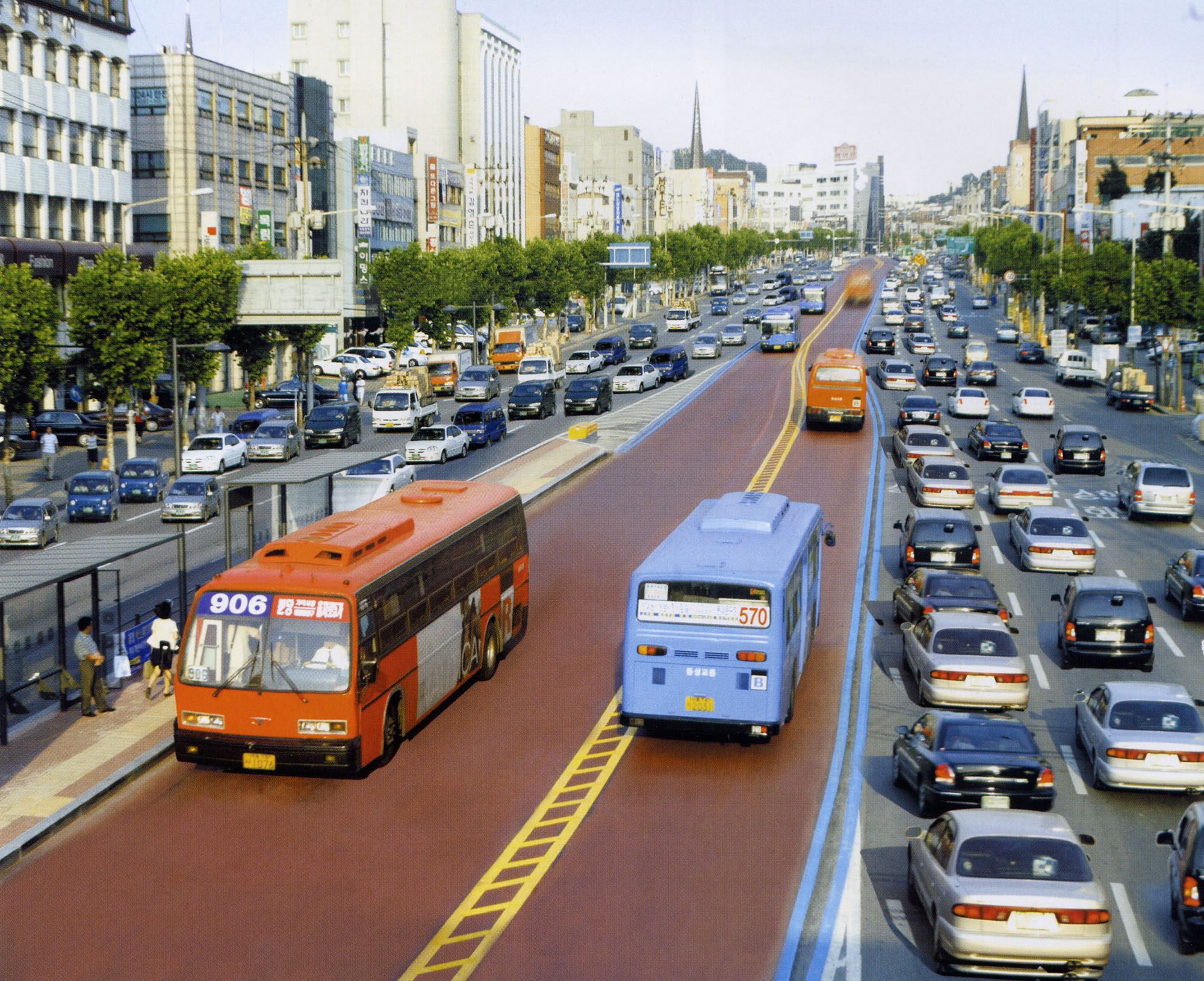
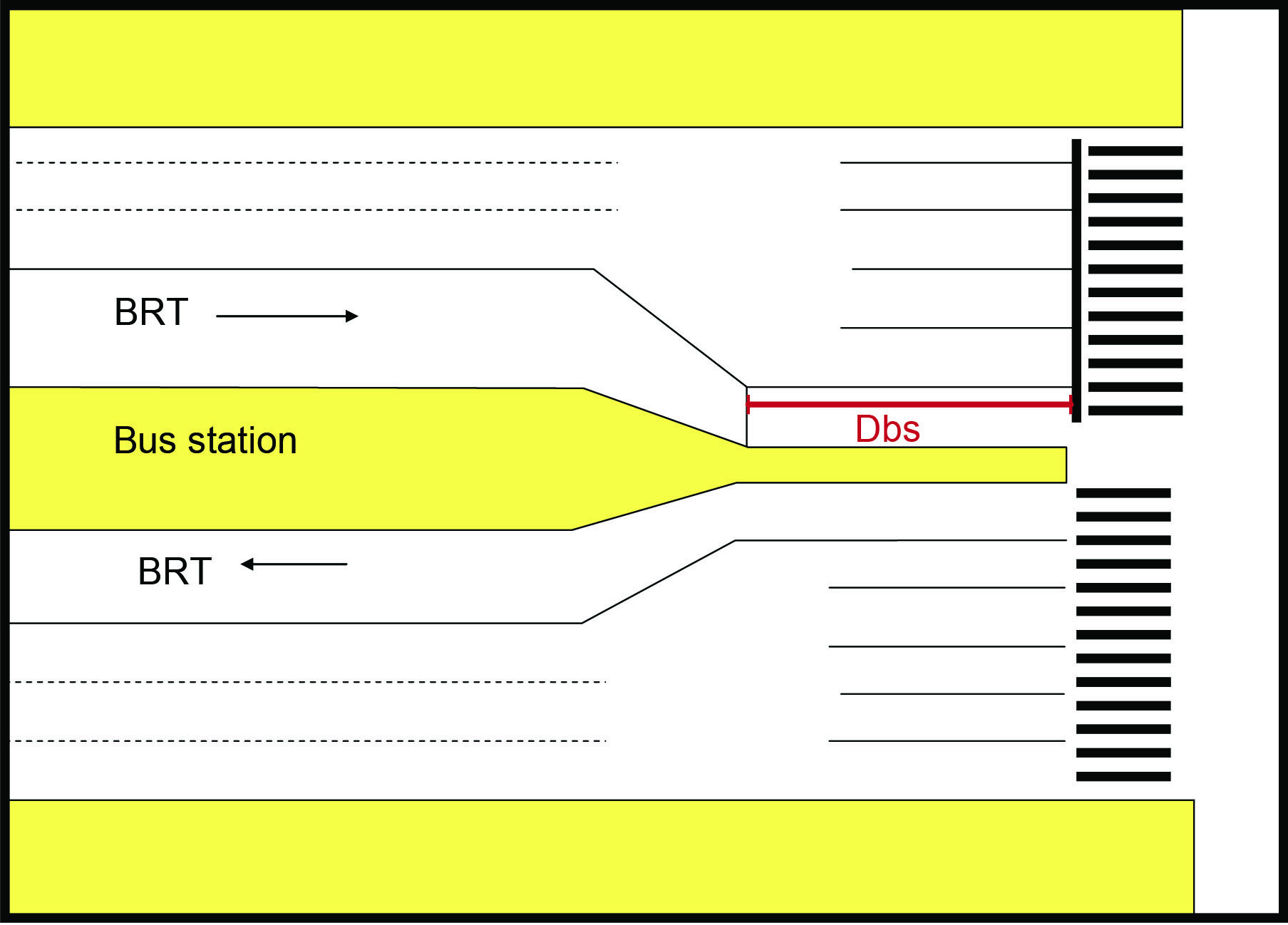
Another compelling reason for separating the station and the intersection is that it minimizes the risk that BRT vehicles will be backed up at the station, which will inhibit the functioning of the intersection and the functioning of the station. If these two potential bottlenecks are co-located, the risk of mutual interference between the station and the intersection increases. Consequently, it is advised to include a safety buffer in the station design for those stations to be located near a signalized intersection. This additional length will temporarily hold buses that: (1) in case of a blockage have cleared the station but are forced to queue up at the intersection until the conflict is resolved, or (2) have cleared the station during the red phase and have to wait for the green phase (Figure 24.25 and Figure 24.26). This buffer should also be around a hundred meters, as the following equations show.

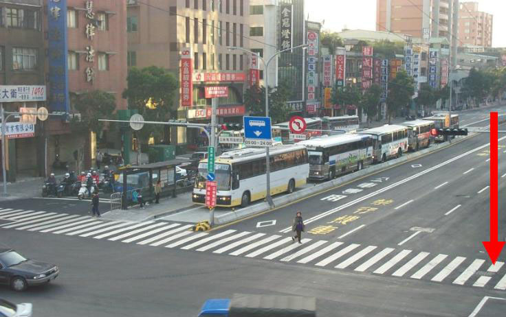
This problem is still serious in “open” BRT systems without clearly designated stopping bays, as bus queueing can be longer than the platform. Besides that, such systems can cause a chaotic boarding process that not only creates stress for the customer but also increases boarding times (Figure 24.27).

The buffer size (Dist_{station-intersection}) should be the space required by queuing BRT vehicles.

\[ \text{Dist}_\text{station intersection} \geq N_\text{vehicle} * \text{Length}_\text{vehicle} \]

Where:

• \( \text{Length}_\text{vehicle} \): Average length of lane space consumed by the queuing BRT vehicles; adding two values:

  • Length of the BRT vehicle;
  • Length of space between BRT vehicles when stopped (usually assumed to be 1 meter).
• \( N_\text{vehicle} \): Likely number of vehicles to queue during the red phase (\(T_\text{red}\)) of traffic signal, discussed below.

Assuming BRT vehicle frequencies (\( \text{Freq}_\text{bus}\)) are 50 percent below the BRT lane saturation flow (\(\text{SaturationFlow}_\text{bus}\)) – that happens practically always, as this represents 360 articulated buses per hour that would carry more than 40,000 customers per hour per direction – \( N_\text{bus} \), which is equivalent to the height of the upper graphic in Figure 24.7, can be determined by:

Eq. 24.20

\[ N_\text{vehicle} = {T_\text{red} * \text{Freq}_\text{vehicle} \over ({1 - \text{Freq}_\text{vehicle} \over \text{SaturationFlow}_\text{vehicle} })} \]

Where:

• \( N_\text{vehicle} \): Number of vehicles;
• \( T_\text{red} \): Time given by a red light holding traffic from crossing an intersection;
• \( \text{Freq}_\text{vehicle} \): BRT vehicle frequency;
• \( \text{SaturationFlow}_\text{vehicle} \): Maximum flow BRT lane can handle;

Example utilizing typical data of an average city in India:

• T_red = 50 seconds (or 50/3,600 hours to use consistent units = 1/72 hour);
• Freq_vehicle = 200 articulated-buses / hour (equivalent to 1 vehicle each 18 seconds);
• SaturationFlow_vehicle = 720 articulated buses / hour (one lane, equivalent to 1 vehicle each 5 seconds);
• Length_vehicle = 19.5 meters (18.5 meters + 1 meter).

\[ N_\text{vehicle} = {{50 \over 3600} *200 \over 1 – (200 / 720)} = 3.8 \text{vehicles} \]

Because one cannot actually have 3.8 buses queueing, \(_\text{Nvehicle}\) must be rounded to the nearest integer, so it is equal to 4.

\[ \text{Dist}_\text{station-intersection} \geq N_\text{vehicle} * \text{Length}_\text{vehicle} \]

\[ \text{Dist}_\text{station-intersection} \geq 4 * 19.5 \]

\[ \text{Dist}_\text{station-intersection} \geq 78 \]

Thus, the minimum recommended distance between the BRT station and the intersection would be 78 meters.

BRT systems currently in operation prove that mixed traffic misbehavior is a relevant source of operation disruptions throughout the public transport system. Traffic spillbacks are commonly seen in heavily congested intersections blocking perpendicular movements along the BRT corridor, so it may be proper to analyze the tolerance; space needed is proportional to red time.

24.4.5Optimizing Walking Distances

As mentioned in the introduction to this section, the willingness to place a station close to the intersection under the excuse of reducing walking times is rarely based on data. In the rare case of low-density areas with few clear origin-destinations where demand is known, the optimal spot can be easily determined. Such locations are not likely to be near busy intersections, and in the event that they are and the intersection is clearly the best location from the perspective of reducing walking time, it is more likely that it is better to move the station back at the length of a few buses than risk hindering the station. That can be perceived considering only the customer that intends to alight in that location: he or she may need an extra minute to walk to the intersection and would need an extra minute inside the vehicle stuck in the station because the vehicle in front is waiting for the green signal. If we consider that all the other customers not alighting there will increase their travel time by one minute and that the queue is likely to get longer (and everyone will wait more than one minute), then it is clear that the station should be moved away from the intersection.

The previous paragraph makes clear that, in high-density areas, to optimize station location with high precision requires labor-intensive, site-specific surveys, and analysis of the origins and destinations must be performed taking into consideration a pedestrian path network encompassing an area within a radius of one thousand meters or more from the possible extremes where the station can be placed. Additionally, several different street crossings should be looked at as well as the placement of other stations. That is, make the simulation model detailed to the level that every block face is a centroid, if not every address.

Our limited experience with such endeavors on central areas has shown that moving a station within a range of two hundred meters has no noticeable effect. But It should be remembered that changing the number of stations within a given corridor extension has a significant impact on overall travel time; that impact is determined by the average distance between the stations as discussed in Chapter 7: Capacity and Speed and requires a much less detailed survey and analysis.

Correction Factor for Station Saturation at Traffic Light

Chapter 7: Capacity and Speed discusses at length the level of saturation of the station, or the proportion of time that BRT vehicles are blocking the station. In particular, mid-block stations are likely to be accessible by at-grade crossings right in front of them. It is generally advisable to investigate the degree to which this intersection increases the saturation of the station.

Roughly, the combination of the station’s normal saturation (which we will call Xstation) and the additional saturation caused by traffic signal interference will reveal the degree of busway saturation. As a general rule, it is best to design the station with a saturation level of under 0.4 at the station, meaning that the station is occupied only 40 percent of the time.

A correction factor that estimates what would be the new level of saturation of the station if the traffic light is positioned right in front of it (X_is0) can be expressed in function of:

• Signal cycle time (\(T_\text{cycle}\));
• Signal red time for the BRT approach (\(T_\text{red}\));
• Average stop time per bus in the station composed by dwell, boarding, and alighting times (\(T_\text{station}\)).

Correction for a Long Red Phase (T_station < T_red)

The relation between Tred and Tstation is the most important; the concern about interference is most acute when the bus stopping time (TB) is short and the red phase (TR) is longer, or of a similar magnitude. Interference is only of limited concern if the red phase is very short.

In this case, to calculate the saturation of the station when faced with interference from the traffic signal, the following formula can be used:

Eq. 24.21

\[ X_{is0} ={ X_\text{station} * T_\text{cycle} \over T_\text{cycle}- T_\text{red} + 0.5*TB } \]

Where:

• \( X_\text{is0} \):Correction factor that estimates what would be the new level of saturation of the station if the traffic light is positioned right in front of it;
• \( X_\text{station} \): Station’s normal saturation level;
• \( T_\text{cycle} \): Time given by the signal cycle;Tred = Time given by a red light holding traffic from crossing an intersection;
• \( TB \): Bus stopping time.

Correction with a Short Red Phase (T_station ≥ T_red)

If the red signal phase is very short relative to the boarding and alighting time, then even if the signal changes to red just as boarding and alighting has been completed, it will be a short time before the light is green again. Thus, there is less concern about interference between the station and the intersection.

Eq. 24.22

\[ X_{is0} = {X_\text{station} *T_\text{cycle} \over T_\text{cycle}-{T_\text{red}^2 \over 2 * T_\text{station}} }\]

Where:

• \( X_{is0} \): Correction factor that estimates what would be the new level of saturation of the station if the traffic light is positioned right in front of it;
• \( X_\text{station} \): Station’s normal saturation level;
• \( T_\text{cycle} \): Signal cycle time;
• \( T_\text{red} \): Signal red time for the BRT approach;
• \( T_\text{station} \): Average stop time per bus in the station composed by dwell, boarding, and alighting times.

Examples

1. Calculating station to intersection interference with a long red phase

\( X_{is0} ={ X_\text{station} * T_\text{cycle} \over T_\text{cycle}- T_\text{red} + 0.5*TB } \)

• X_station = 0.35;
• T_cycle = 700 seconds;
• T_red = 500 seconds;
• T_station = 10 seconds.

\[ X_{is0} ={ 0.35 * 700 \over 700 \text{seconds} - 500 \text{seconds} + 0.5* 10 \text{seconds} } = 1.195 \]

In this hypothetical example the station would operate on just the 200 seconds of green, but not on the 500 seconds of red, because just some seconds after the red phase begins the bus will finish boarding, but it will obstruct access to the bus stop during the entire 500 seconds of red. Thus, at a value of 1.195 the high saturation leads to considerable congestion of the busway.

2. Calculating station to intersection interference with a short red phase

\( X_{is0} = {X_\text{station} *T_\text{cycle} \over T_\text{cycle}-{T_\text{red}^2 \over 2 * T_\text{station}} }\)

• \(X_\text{station} = 0.35\);
• \(T_\text{cycle} = 30 \text{seconds full signal phase}\);
• \(_\text{Tred} = 15 \text{seconds of red phase}\);
• \( _\text{Tstation} = 40 \text{seconds of vehicle stopping time}\).

\[ X_{is0} = {0.35 * 30 \over 30 - {15^2 \over 2 * 40} } = 0.386 \]

In this case, because the red phase is quite short, there is fairly minimal risk that the traffic signal will disrupt the functioning of the bus stop, so saturation increases only marginally, from 0.35 to 0.386.