6.2Basic Data Collection
It is a capital mistake to theorise before one has data. Insensibly one begins to twist facts to suit theories, instead of theories to suit facts.Sir Arthur Conan Doyle, writer and physician, 1859–1930
In order to propose an optimal service plan, its costs and benefits must be known, and understanding customers’ needs is essential for achieving that. The current state of the public transport system may not exactly show all user demands, but it will certainly point in that direction more reliably than alternatives; it is composed of very objective and comprehensive information, which is cheap to collect in comparison with alternatives and overall project costs.
While existing public transport operations are sometimes poorly aligned with public transport customer needs for a variety of reasons, in most cities economic forces tend to push public transport services close to consumer needs. In addition, customers are used to the services as they currently exist—and resist change. Service plans should be developed conservatively, moving away from existing services only when compelling data indicates that a change would improve services.
Ideally, the data collected should be enough to understand all existing services, the demand throughout the day, and the full trip origin and destination for every public transport customer in the corridor influence area, or at least the time and location of where customers entered the existing public transport system and where they exited.
Normally, this does not require having all the data about every trip, but rather having a sample of data large enough to infer the behavior of the whole. Even where all disaggregated trip data is available, as well as a computer program able to process it trip by trip (to date, no current demand modeling software has such capabilities), a systematic aggregation is still necessary so that the results can be analyzed by humans.
The common way of doing this is to provide customer demand information aggregated per hour of the day in a visual format. It is always best to have data for both peak and off-peak periods. For the analysis in this chapter, much of the services and engineering will be designed around the peak hour, so an estimated peak hour demand is needed. If the frequency is very low, it may be necessary to aggregate by peak period, as in morning peak, midday off peak, afternoon peak, and so forth, and then infer the average peak hour demand from the peak period, in order to avoid data distortions. For instance, in the United States, a bus route might have only three trips between seven and eight, and only two between eight and nine, because one of the trips falls at 7:59 and one falls at 9:01, creating a false impression that demand is far more irregular than it is. In general, however, the data needs to be put in a “peak” hour format, as this is used to make key engineering decisions. Business planning decisions must also be informed by the relationship between the peak hour and the off-peak periods, as this relationship can make (or break) the financial sustainability of the project.
For service planning, the following data is needed:
- The itinerary of every route,
- The number of departures per hour;
- The average travel time between stops;
- The number of customers boarding and alighting at each stop;
- The number of customers transferred from each route to every other route.
Initially, it is only relevant that this data is processed for typical days, but when the project moves forward, service plans for Saturdays and Sundays and seasonal variations (school holidays) will be required for a complete evaluation. Additional trip data, as described below, may already have been collected using the methods described in Chapter 4: Demand Analysis, and repeated here, focusing on the processing needs for the service plan design.
6.2.1Itineraries and Average Travel Time between Stops
For the process of corridor selection, all of the existing public transport routes using the planned BRT corridor should have been mapped into a GIS program (or a GIS interface of a demand modeling tool like TransCAD or Emme).
If this information is not already available, or badly coded, it will be necessary to have surveyors ride each bus with a GPS and record the coordinates of each bus stop and each bus route. This is not expensive or difficult. Even if this data has already been collected by someone else, it may be out of date, so it is a good idea to check the data by randomly sampling the key routes with a GPS to make sure it is accurate. Many software applications (apps) for smartphones can collect this data.
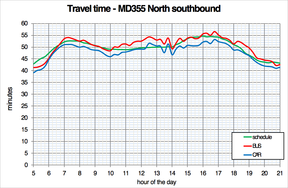
Average speeds from bus stop to bus stop should be surveyed during the peak hour and off-peak period. For a given distance, a graphic such as the one below can be generated to represent the speed over the course of a day. Data needs to be collected over multiple days to generate a reliable average speed.
In a growing number of cities, the bus routes have already been input into an open standard format like General Transit Feed Specification (GTFS) that allows people to manipulate the data in multiple applications. Usually this data is used for customer information dissemination (its name was originally Google Transit Feed Specification), but these same data sets can be used for service planning. GTFS data may be good enough to give coordinates for mapping the existing public transport system, or it may have a lot of inaccuracies that need to be cleaned up. The route needs to be mapped in both directions, as buses may not take the same route going in different directions and bus stops have different positions.
6.2.2Number of Customers Boarding and Alighting at Each Stop
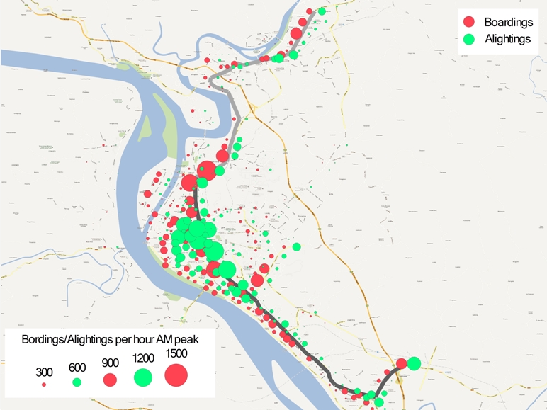
The number of existing bus or minibus customers that are currently boarding and alighting on all of the bus routes that use the BRT corridor at each station needs to be collected and mapped. This is usually done by a survey team. Typically, along the planned BRT trunk corridor, if the stations are clearly marked and used, the boarding and alighting counts can be conducted at the stations. For the parts of bus routes that extend beyond the trunk corridor, boarding and alighting counts are generally conducted on board. If the buses or minibuses do not stop in consistent locations, the boarding and alighting numbers along a link need to be collated and assigned to a reasonable location or segment approximating most boardings and alightings, or a location where a new BRT station is being considered could also be used. Boardings and alightings are typically known within a segment, but not at an exact location.
Sometimes boarding and alighting numbers can be collected from Automated Passenger Counter (APC) systems if the locale has this technology. APC data can sometimes give very detailed and accurate numbers of boarding and alighting customers per bus route, but frequently they are coded by time of day, and the station location is not fully clear, so a correlation between APC and existing stops needs to be determined.
With this data, a map such as the shown in figure 6.2 should be generated:
This data can already be used to identify some stations that could possibly be eliminated in the new BRT service, or stations that might become express stops. In the United States, there has been a tendency over the years to accommodate citizens’ demands for adding additional stations to the point where there are stations every 200 meters or less. If a stop has very few customers boarding or alighting, extra delay is being imposed on all the customers on board the bus to accommodate only a handful of people. The BRT Standard imposes a deduction of 2 points for station stops closer together than 200 meters. In some of the high-demand BRT systems in Asia and Latin America, stations are sometimes 200 meters long. In addition, this data is used to identify locations where off-board fare collection may be the most important.
Further, it is used to identify important transfer nodes. Where large boarding and alighting volumes are observed in locations with perpendicular public transport routes and no other clear destinations, it is likely that many of the customers are transferring. Identifying these transfer points is important to service planning, and additional surveys will need to be conducted at these transfer points as discussed in the next subsection.
6.2.3Number of Customers Transferring between Routes
The boarding and alighting data can be used to either construct and/or calibrate a public transport trip origin-destination (OD) matrix. This public transport OD matrix reveals where public transport customers want to go, regardless of where the current bus or minibus routes go. It can be developed in a number of ways depending on the sort of data available.
For a single corridor, when there is no other data, modelers typically use the same boarding and alighting counts done above to first create a “stop-to-stop” OD matrix for routes serving the selected BRT trunk corridor. This is generally done by a Fratar distribution model. This mathematical method makes assumptions about where people are getting on and off public transport vehicles based on uniform probability. This data will generally reliably re-create where customers are starting and stopping their journeys along a single public transport route, but it misses where customers may be transferring to other routes.
In order to transform the stop-to-stop OD matrix into an OD matrix for full trips along the pilot BRT corridor, transfer surveys that identify not only the number of people transferring but also their final destinations need to be conducted where large volumes of customers board and alight or at locations that intersect other public transport routes. All major likely transfer points should be surveyed. Many systems, however, have large numbers of transfers distributed across the entire corridor and not necessarily concentrated at particular stops, so it is harder to create a full public transport OD matrix from this methodology alone.
The transfer survey should interview a statistically significant sample of the boarding and alighting customers at each stop and ask them their trip origin, destination, and the public transport route they used to make the trip. Once this data is collected, the stop-to-stop OD matrix should be modified based on the transfer survey data, to link the appropriate proportion of stop-to-stop trips based on the transfer survey results.
In the developed world, there is usually more data available than can be easily processed. For instance, in the United States, a growing number of cities are creating public transport OD matrices from new ticketing system information. A growing number of public transport ticketing systems can track by ticket ID number where a customer enters the system (where he or she swipes at a payment site). By noting where he or she enters the system next, usually in the evening from his or her destination or at some transfer point, one can create a matrix of trip origins and destinations for virtually all public transport customers. All of this is used to generate a detailed customer “origin and destination matrix.”
After this is done, there is sufficient data in the demand model to test alternative service plan scenarios. If put into a public transport demand model like TransCAD or Emme, more refined alternative service planning options can be developed and tested.
6.2.4Data Processing
For each existing bus or minibus route along the selected trunk corridor, as stated above, data of existing operations needs to be collected for the full length of daily operations. Then, the following information can be generated for assisting the service plan:
- Total route distance;
- Route travel time: total, disaggregated by section and hour of day per section;
- Stop-by-stop boarding and alighting customers;
- Vehicle loads at each link (between each station);
- Overall public transport vehicle and occupancy per section;
- Overall public transport vehicle frequencies.
From this data, the critical link and load of the corridor can be identified, also known as the maximum load on the critical link (MaxLoad). At this location, it is important to have full-day public transport vehicle and occupancy counts with consistent data.
From the full-day counts at the critical link, the degree to which the demand has peaked on the corridor can be calculated. This is needed in order to calculate the required fleet under different scenarios and to convert peak hour ridership numbers to daily numbers. The total route distance and link-by-link peak hour speed are needed to calculate the route-by-route full-circuit total cycle time (TC).
Though not completely necessary at this stage, it will also be useful to know:
- The existing fleet size;
- The total customers per line per day and per peak hour (to calculate the renovation rate [\(Ren\)]);
- The total vehicle distance operated on the route.
It will also be necessary to calculate:
- The total amount of the route that overlaps the corridor;
- The total cycle time that occurs on the planned corridor and off the planned corridor.
This information gives us the preliminary tools to begin a service planning analysis.
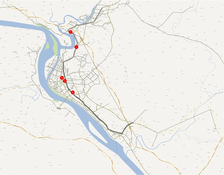
As an example, Figure 6.4 shows a corridor identified as a future BRT corridor in Montgomery County, Maryland, USA, to which the involved routes are shown in Figure 6.5. The Table 6.1 presents the total amount of the route that overlaps the corridor, and the part of total cycle time that occurs on and off the planned corridor.
Figure 6.6 shows travel time differences with the BRT speeds (the pink line) and with the current speeds (red line) and the benefit per trip in minutes (the difference between the lines) for the route to be incorporated into the BRT corridor in each period of the day. Off-peak benefits will be smaller. The potential benefits of implementing each alternative are calculated in table in figure 6.6 for the proposed preliminary service plan by multiplying the number of customers for each trip throughout the day by the estimated travel time saved.
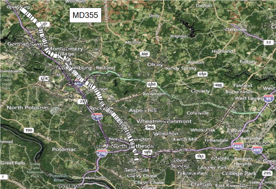
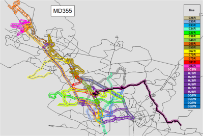
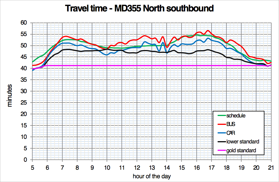
Table 6.1Existing bus routes using the Route 355 proposed BRT corridor, proposed changes for two scenarios and time savings for Montgomery County, Maryland, USA.
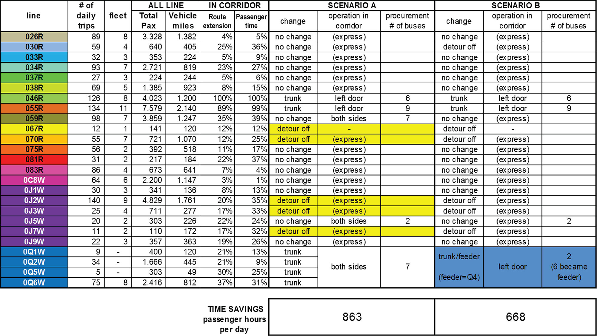
In Table 6.1, which was generated for Montgomery County using the GTFS and APC data corresponding to the routes in Figure 6.5, route extension is the percentage of the bus route that overlaps with the proposed BRT corridor, and passenger time is the percentage of the customer’s time that is the spent on that section of the bus route that overlaps with the proposed BRT corridor. While these two indicators essentially measure the same thing, the comparison between the two allows for identification of congestion and thus where BRT would significantly improve travel times. If the customer time in the corridor (last column marked “passenger time”) is higher than the percentage of full bus route length that overlaps with the BRT corridor (second to last column named “route extension”), this indicates that the corridor is where most of the congestion is, which suggests BRT should help significantly improve travel times.