6.3Basic Service Planning Concepts
When I was young, I had to learn the fundamentals of basketball. You can have all the physical ability in the world, but you still have to know the fundamentals.Michael Jordan, former professional basketball player, 1963–
6.3.1BRT Stations and Saturation
With rail systems, the constraint on capacity tends to be the frequency that the signaling system can handle. Rail system designers thus frequently try to add longer and longer trains, but on city streets eventually this runs up against block lengths. In BRT systems, by contrast, the constraint on capacity is the BRT station. Vehicles can platoon, in which many can follow very closely, one behind the next, with very high frequencies. A traffic signal can handle far more vehicles passing through it over the course of an hour than a bus stop can process. As a result, for BRT, the station saturation problem is the critical issue that needs to be solved to maintain system speeds—not intersections or headways, which can be defined as the time between two vehicles offering a service, conveying exactly the same information as frequency.
Thus understanding the saturation level of a station is a basic starting point in achieving high capacities and high speeds (covered in the next chapter), and if there is a risk of station saturation it also becomes a primary concern of service planning (covered in this chapter). Saturation level of a station refers to the percentage of time that a vehicle stopping bay is occupied. The term saturation is also used to characterize a roadway, and in particular, the degree to which traffic has reached the design capacity of the road.
When engineers talk about the capacity of a road or a BRT system, they will give a capacity for an acceptable level of service, rather than for the maximum number of vehicles or customers that could pass through a road or a system. After a certain point, the lane or BRT system becomes congested. With congestion, the total flow of vehicles may not change (usually it increases at first and later decreases), but the vehicles are going slower and slower.
Saturation, of course, changes as the demand (arrival of vehicles) is not perfectly regular; so when we talk about saturation we are assuming a permanent flow subject to the irregularity normally observed in a roadway or in a busway. The peak hour is an appropriate measure of saturation for dimensioning a system.
Exactly because of this irregularity, a level of saturation of (x=) 0.85 is commonly considered acceptable for mixed traffic. Below a saturation level of 0.85, increases in traffic will have only a minimal impact on average speeds, and the level of service is acceptable. Once saturation levels exceed 0.85, there is a dramatic drop in speeds.
However, with BRT stations, there is no clear breaking point. The queues and delays at bus stations occur at small amounts even at low saturation levels, and these delays simply increase with saturation. In the case of a bus station, saturation is defined as the percentage of time that the station is occupied by vehicles boarding and alighting customers.
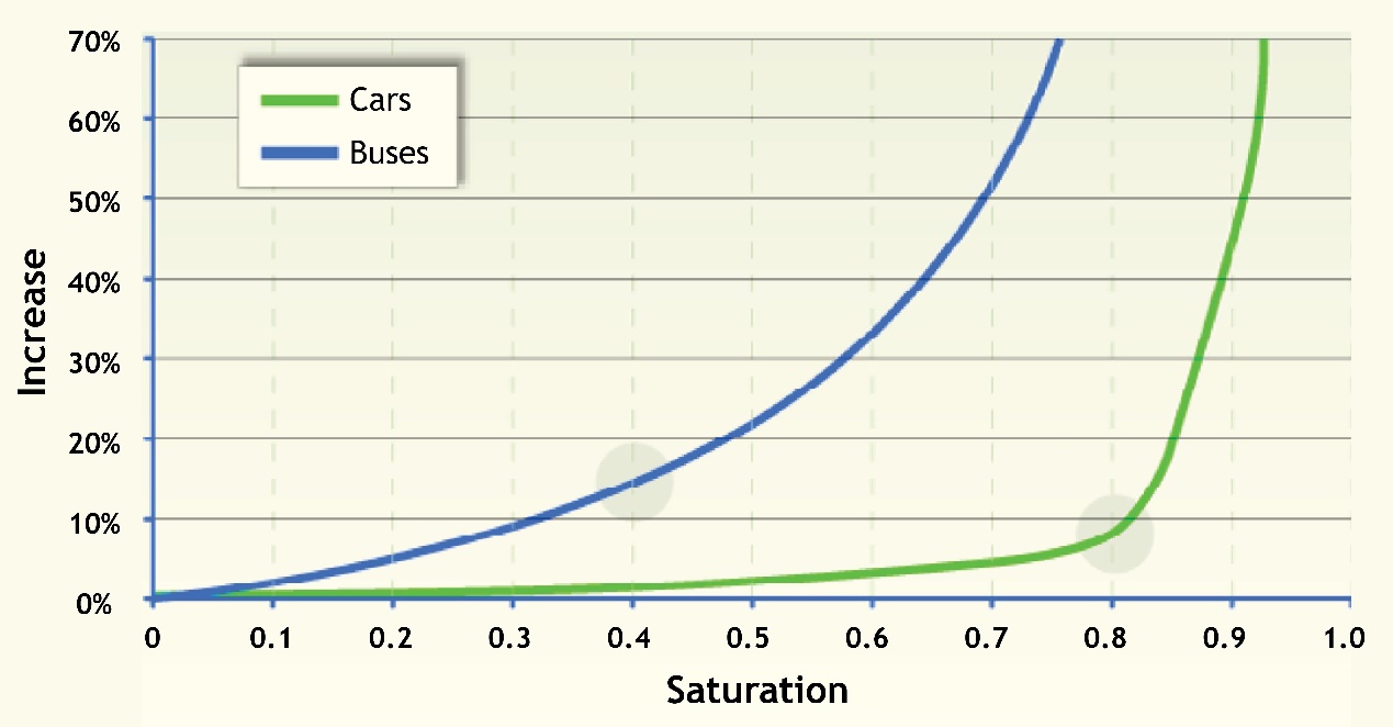
In general, stations should be planned at less than 40 percent saturation, or else the risk of congestion increases significantly. The impact of stopping bay saturation on speed is shown in Figure 6.7.
Rather than a clear point at which the system collapses, station saturation tends to lead to a gradual deterioration of service quality. For this reason, the optimum level of station saturation is not clear. Some studies argue that the optimum should be around 0.30, but saturation levels as high as 0.60 can be tolerated in specific locations if this condition is not general throughout a BRT corridor. However, for saturation levels above 0.60, the system can be deemed unstable, and risk of severe congestion and system breakdown is considerable.
A low saturation level, or a high level of service, means that there is a low likelihood of vehicles waiting in a queue at a BRT stop. A high saturation level means that there will likely be long queues at stopping bays. For saturation levels over one (\(x > 1\)), the station will certainly have queues increasing to the point where the system does not move until long after the peak is over.
6.3.2Sub-Stops and Docking Bays
A docking bay is the designated area in a BRT station where a vehicle will stop and align itself to the boarding platform. Docking bays are typically aligned quite close together, so close in fact that one vehicle does not have the space to pull around and pass another vehicle stopped in front of it at another docking bay.
Sub-stops, by contrast, are the stopping areas where one or more docking bays may be located. A station may be composed of more than one sub-stop. The critical thing about a sub-stop is that it be far enough away from the next sub-stop that any vehicle pulled up to a docking bay in the sub-stop in front of it has enough space to pull around and pass the other vehicle. This requires that one BRT vehicle be able to pass another BRT vehicle at the sub-stop, which necessitates a passing lane. Because sub-stops and passing lanes are extremely critical to avoiding station saturation and hence reaching higher speeds and capacities, and making express and limited stop services viable, they are both given points in The BRT Standard.
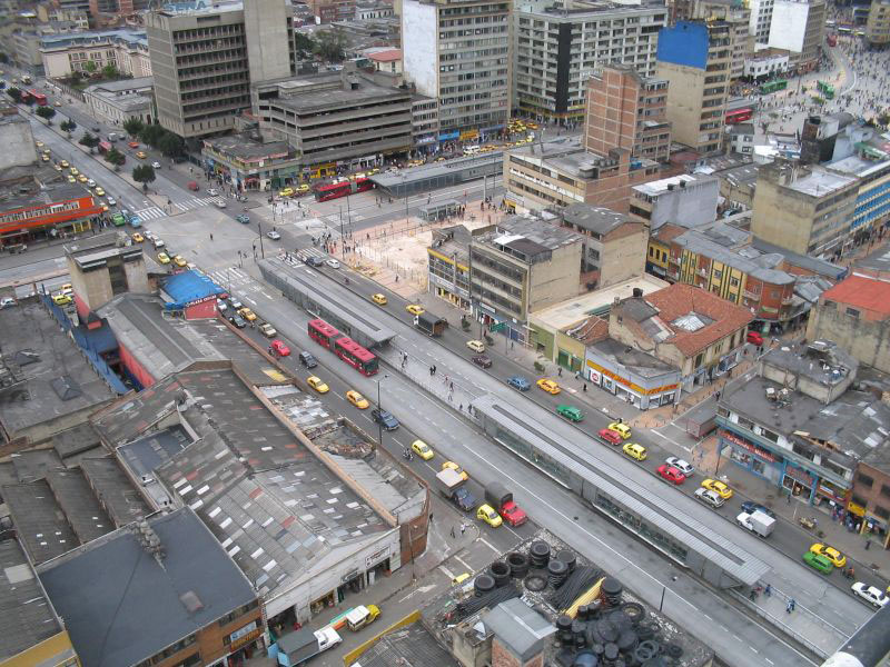
In the first BRT systems, each station had only one docking bay and one sub-stop. A key innovation of Bogotá’s TransMilenio system was that more capacity and speed could be obtained, if, at each station, instead of having just one sub-stop with one docking bay, each station might have two or more sub-stops, and each sub-stop might have one or two docking bays. In Figure 6.8 the TransMilenio stop has two sub-stops, one with one docking bay and one with two docking bays.
By adding more sub-stops and docking bays (the sub-stops are far more important than the number of docking bays), the saturation level of each sub-stop can be kept to a maximum value of 0.40 until very high levels of demand are reached. TransMilenio strives to keep the maximum variation in the saturation value at no more than 0.10 between sub-stops at the same station, so the values should not vary from a range of 0.35 to 0.45.
6.3.3Direct Services
Direct services, sometimes called “trunk extensions” or “complementary” routes, are new BRT services that operate both in mixed traffic and inside dedicated BRT infrastructure on trunk routes. Usually, they follow former bus or minibus routes that have been converted into BRT services.
When designing BRT services, the easiest thing to do is to simply convert existing public transport routes into identical new BRT routes, and allow whatever portion of the existing route that does not overlap with planned BRT infrastructure to simply operate in mixed traffic. One of the main advantages of BRT over rail-based modes is that buses, unlike rails, can easily leave the trunk infrastructure and operate on any normal road.
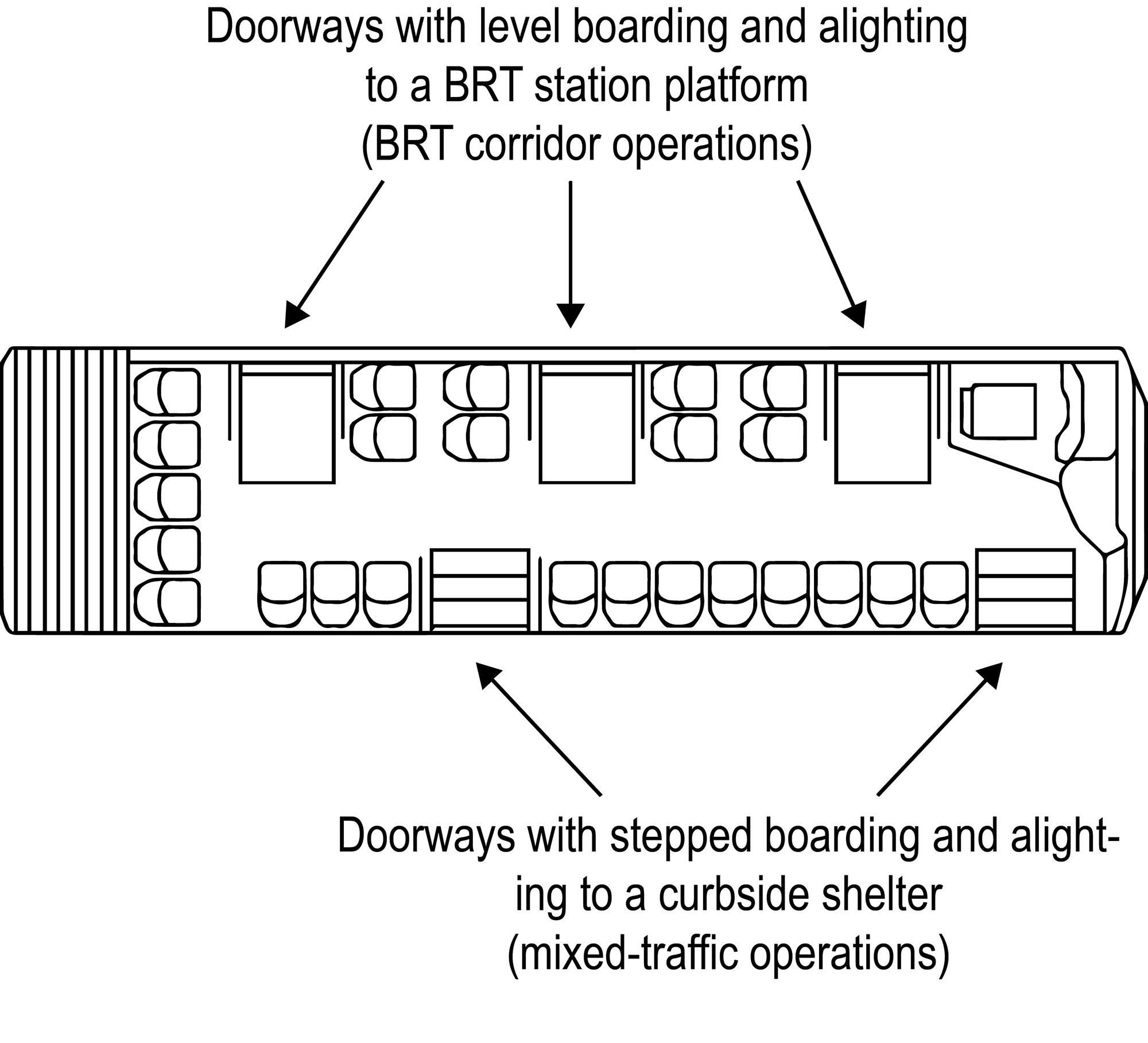
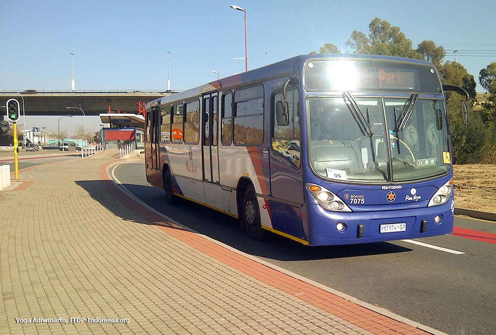
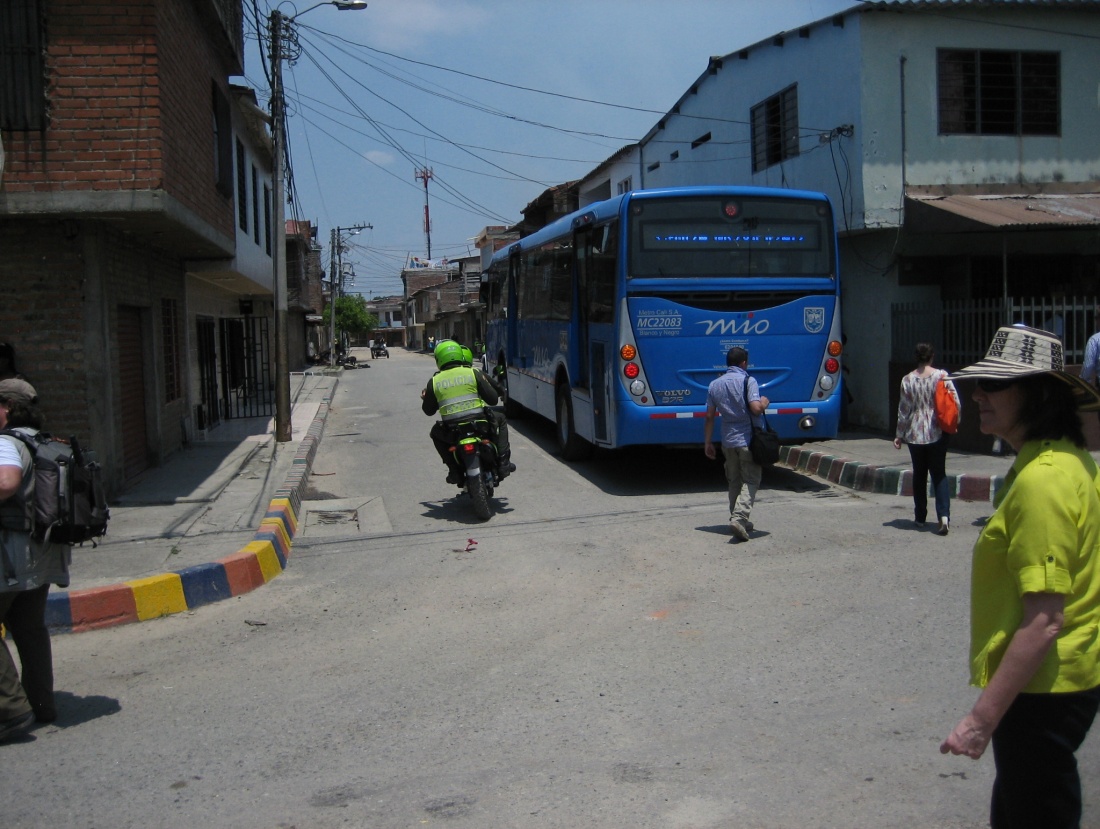
If a city has already done a good job designing its bus services, and the routes are well correlated to trip origins and destinations, it may be a good idea to leave several or most of them more or less where they are. Riders are already familiar with these routes, and a conservative approach to BRT service planning will minimize the likelihood of major mistakes or public confusion when the new system opens. Because such routes need to operate both in mixed traffic and along specialized BRT trunk infrastructure, the buses and the fare collection system need to be able to operate in both environments. Generally, this will require the procurement of a fleet compatible with the new BRT infrastructure and mixed traffic operation. Developing BRT vehicle technical specifications that allow for both BRT trunk and mixed traffic operation (see Figure 6.9) significantly improves the flexibility of the system. If the system has central median platforms on the BRT trunk corridor, vehicles will need to have doors on both sides. Direct service systems increasingly use low-floor buses to ease boarding and alighting off the trunk corridor. Direct service operations with flexible vehicles also make it easier to expand BRT trunk infrastructure onto other linked corridors without major disruptions in service or new fleet procurement. Direct services within a closed system can employ off-board fare collection at BRT stations, but need to have an on-board or proof-of-payment fare collection system when using regular bus stops outside the BRT corridor. With proof-of-payment systems, inspectors will be needed, and there is risk of fare evasion.
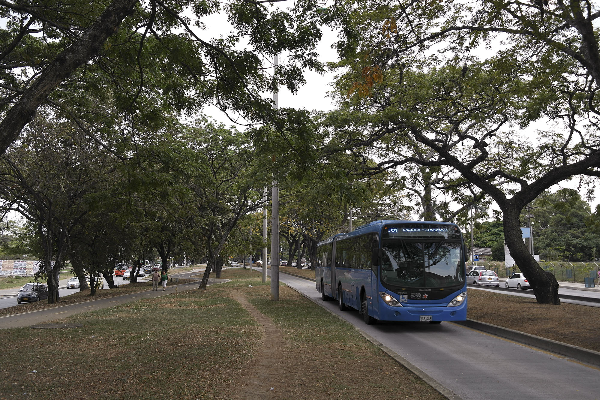
Until 2010, the only direct-service BRT reaching Silver or Gold Standard was the Brisbane Busway (Australia). Many of the Bronze-rated BRT systems with direct services lacked basic administrative controls over access to the trunk BRT infrastructure, with lower quality vehicle infrastructure improvements, and these systems frequently encountered station saturation problems. Problems of station saturation are not caused by direct services, but rather by a misalignment between the service plan and the infrastructure design that could happen regardless of service type. Since 2010, several systems have opened (Guangzhou, China; Cali, Colombia; Johannesburg, South Africa) that feature Gold- or Silver-Standard BRT infrastructure and direct services. These systems all offer services that operate both on Gold- or Silver-Standard BRT trunk infrastructure and continue beyond the trunk into mixed traffic.
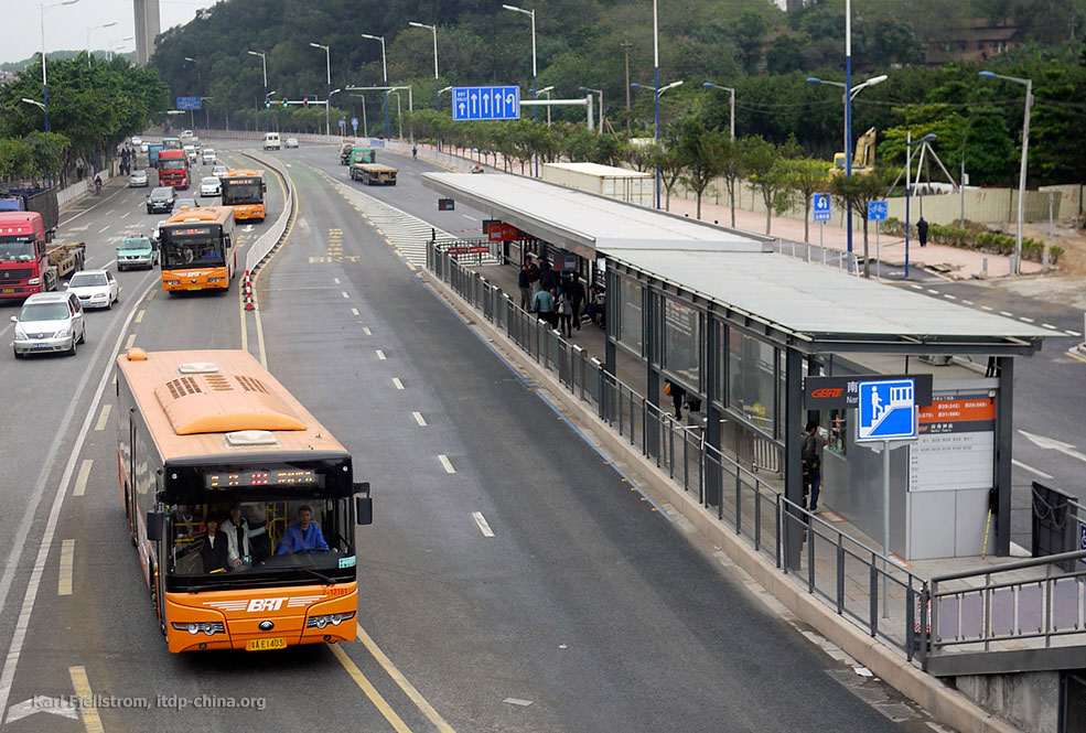
Guangzhou’s BRT proved that direct services in a closed system with Gold Standard BRT infrastructure and properly sized stations can reach very high capacity and speed with high customer service levels. Guangzhou’s peak-hour, single-direction passenger flows, at over 27,000 passengers per hour per direction (PPHPD), are double all but the best trunk-and-feeder BRT systems in the world.
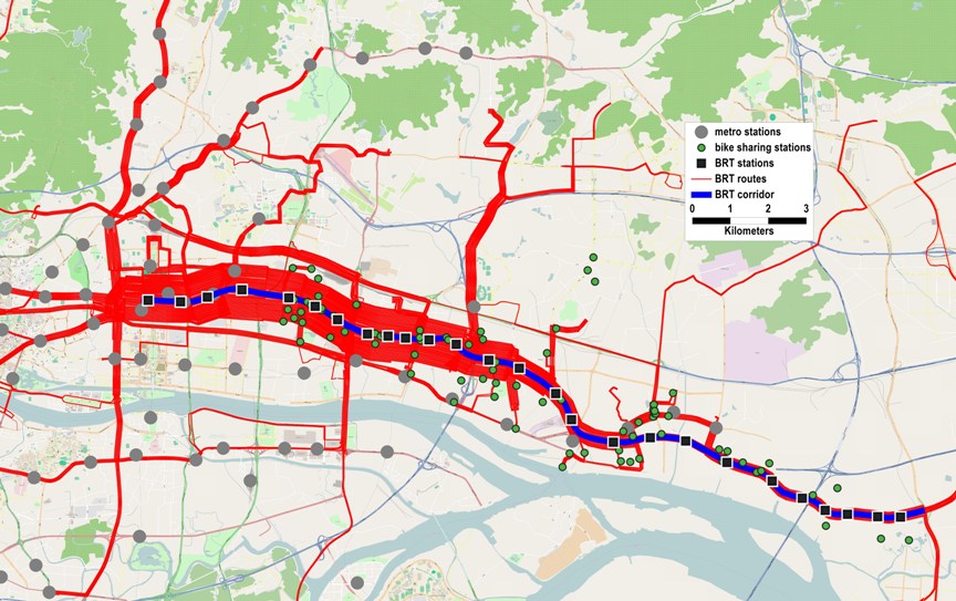
Figure 6.13 provides a map of the services for the Guangzhou BRT system. The BRT routes illustrated in Figure 6.13 are allowed to operate along the BRT trunk corridor. The physically segregated busways and prepaid boarding stations were built along the trunk corridor illustrated in this figure, which also shows the bike-sharing stations implemented along the BRT corridor. Although the trunk corridor is only 23 kilometers long, BRT service coverage extends to 273 kilometers of roadways in the city.
6.3.4Trunk-and-Feeder Services
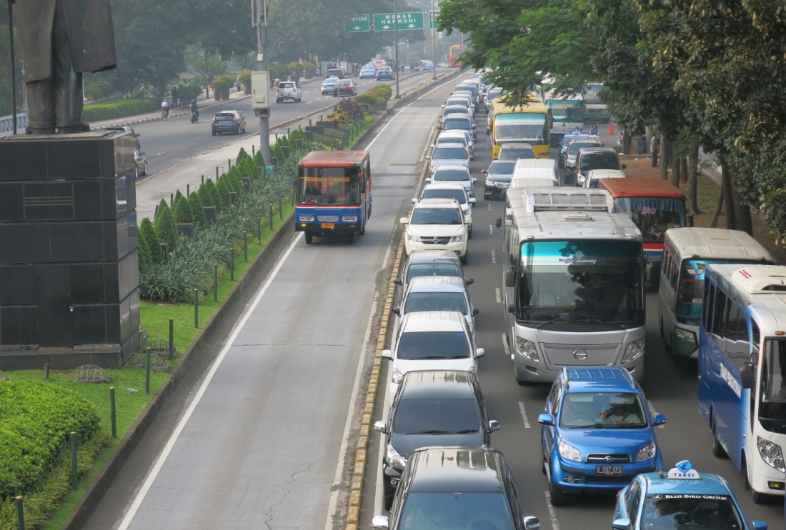
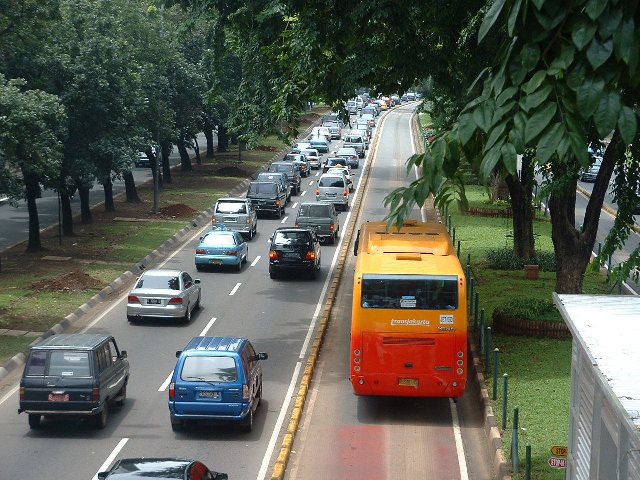
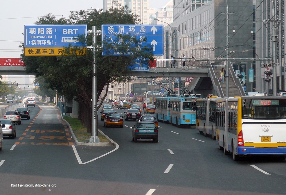
Until recently, the most famous BRT systems operated “trunk-and-feeder” or “trunk-only” services. In some cases, a new BRT service will run only up and down the BRT trunk infrastructure. This would be called a “trunk-only” service. Trunk-only services can either allow the previous routes to continue to operate in mixed-traffic lanes parallel to the BRT corridor, and then continue as the route extends past, or they can be rerouted off the corridor, or they can be eliminated and force their former customers to transfer to the new BRT. The approach of allowing former bus routes to continue in mixed traffic is what occurred in Jakarta, Indonesia, and in many Chinese systems. It has the advantage that it does not force customers to transfer against their will. These systems have the disadvantage that the ridership of the BRT system tends to be lower, undermining returns to scale in the BRT system operation. Also, as it leaves many bus routes in the mixed traffic lanes, this approach also tends to degrade the level of service in the mixed traffic lanes, resulting in lowered mixed traffic speeds due to increased congestion.
Initially, trunk-and-feeder service design was the result of BRT system developers copying the service characteristics of rail systems without considering direct service alternatives that were possible with BRT. Often, designers of “trunk-only” services think that informal operators will automatically provide feeder services to the trunk routes. In some cases, where enforcement and regulation of informal operators is reasonably effective, this can bring some customers to the trunk system, though it normally forces customers to pay twice, and does little to improve the quality of the trip still being performed by the informal part of the service. More typically, however, informal operators will refuse to stop at trunk stations in an effort to retain their customers for the longer haul trip, draining the BRT system of ridership and revenue, and congesting parallel mixed-traffic lanes.
TransJakarta remained for many years a “trunk” system without a “feeder.” As a result, despite being one of the longest BRT systems in the world at over 172 kilometers, in early 2012 it carried only 350,000 customers per day and about 4,000 customers per hour per direction at peak times. Roughly two-thirds of all public transport customers using the TransJakarta corridors continued to use their former bus routes and operate in very congested mixed traffic conditions. While some operational improvements have been made, and a few new direct services have been added, the system has yet to fully optimize its services and operates at a loss.
Mexico City also operates a trunk-only system. Rather than allowing former bus routes to operate in parallel, it cancelled them, reducing mixed traffic congestion and pushing up ridership on Metrobús. The new routing did not cause that many new forced transfers, because most of the former bus routes were already organized to operate on corridors in a manner that was not fully consistent with demand pattern. As the Mexico City system expanded, inter-corridor routes were added, and the system began to serve more customers, while reducing unnecessary transfers and station saturation.
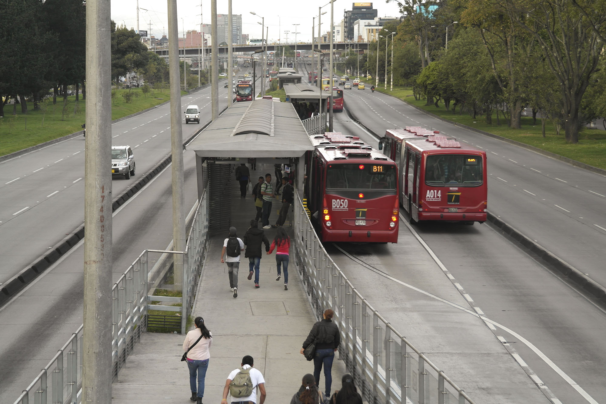
Systems such as Bogotá’s TransMilenio, Curitiba’s system, Rio’s TransOeste/TransCarioca/TransOlímpica, Lima’s Metropolitano, and others provide fully integrated feeder bus services that connect to the trunk services in formal transfer terminals, offering a better quality and more comprehensive door-to-door service than the trunk-only services. In this case, a former bus route that overlaps the trunk BRT corridor for only part of its route is split into two services: a trunk service operating only inside the BRT system, and a feeder route that operates in mixed traffic.
In the best systems, the BRT system operator operates both trunk services and feeder services under professional quality of service contracts with private vehicle operating companies. Such feeder services are not operated by informal operators, but by modern companies, and they form an integral part of the BRT system, with consistent branding, fare systems, information technology, and other BRT amenities. In some cases, especially in higher-income countries, a public transport authority is likely to operate both a BRT trunk service with special vehicles and branding, and a feeder service using normal buses in mixed-traffic lanes that are unlikely to be identified as part of the BRT system.
6.3.5Services That Skip Stops: Limited, Express, Early Return, and Deadheading
The most basic type of public transport service along a corridor is typically known as “local service.” This term refers to a service where stops are made at each station along a route. Thus, while local services provide the most complete route coverage along a corridor, such services also result in the longest travel times and the slowest speeds.
Each stop a vehicle makes adds some delay. One of the easiest ways to increase vehicle speeds is to add services that skip stations. Services that skip a few stations at regular intervals are usually called “limited stop services.” Services that skip many stations are generally called “express services.” One of the main advantages of BRT is that it is relatively simple and inexpensive to allow one vehicle to pass another by simply having passing lanes at station stops.
Single-track metro and light rail transit (LRT) systems and simple, single-lane BRT systems like TransJakarta and RIT Curitiba (except for the new Linea Verde), which do not have passing lanes, have few options but to operate only local services. There are no provisions within the infrastructure of these systems for vehicles to pass one another. Allowing passing in the infrastructure design can provide more service options and is a main reason why The BRT Standard weighs heavily the inclusion of passing lanes in the design.
Many of the examples in this chapter assume that it is possible to build physical infrastructure that can accommodate the passing of one service by another, generally through the inclusion of passing lanes inside the BRT infrastructure. The best solution is to simply provide enough space for passing lanes at station stops. The space is not needed along the entire corridor, only at stations that can be set back from the intersection to avoid compromising intersection capacity. When right-of-way for passing lanes is simply unattainable, figuring out how to accommodate passing to allow longer distance limited and express vehicles to pass local BRT services and still use the dedicated BRT infrastructure is a challenge. A variety of alternatives have been discussed, though with fairly limited application to date. Most of these techniques only work up to a certain maximum frequency.
If the barrier between the busway and the mixed-traffic lanes is not rigid and can be easily permeated, it is possible for express and limited buses to simply pass each other in the mixed-traffic lanes. This is often done in bus system improvements like Select Bus Service in New York, but so far there are no examples of this in full BRT systems. Its effectiveness depends on the degree of mixed traffic congestion at the critical points where the buses need to pass one another.
Another technique is to time services so that limited stop or express services only catch up with the local services at the terminal point of a route, or at select stations where passing lanes are available. Such services, called “catch up” services, are more commonly seen in rail systems. Thus, an express service may begin ten minutes behind a local service, and this starting-time difference ensures that the express service does not overtake the local service. Such an approach may be applicable to BRT for relatively short corridors with relatively long headways (e.g., ten minutes), but to date there is limited experience, and its application has been limited to express-service demands only.
Some cities have considered adding a pull-by bay in front of stations, where a local BRT vehicle can pull aside and let an express bus pass. This solution has the benefit of only requiring right-of-way where it is least needed for other purposes, such as BRT stations or turning lanes. Some preliminary analysis indicated that pull-by bays at some stations might be feasible in systems with headways greater than about five minutes, but there remains limited real-world experience with their application.
If the BRT infrastructure does not include passing lanes at station stops, it may be advisable to leave express services in mixed traffic lanes. Curitiba’s RIT system, for instance, excluded longer-distance express buses from BRT services due to the lack of passing lanes. This was a second-best solution, the benefits of which degraded as traffic congestion increased in the mixed-traffic lanes. One of the main innovations of Bogotá’s TransMilenio was to introduce express, limited, and local services, all inside the BRT infrastructure.
Sometimes the overabundance of stops is mitigated by stop-on-demand. Stop-on-demand does not work well during peak hours, however, as there is usually demand for all of the stops. It is also virtually incompatible with BRT services. Since stop-on-demand offers limited benefits during the critical peak period, and does not integrate well with BRT, it is generally not used in BRT services and hence is not further considered here.
In many developing-nation cities, public transport services operate on a hail-and-ride basis. Even in cities in the United States, minibus services effectively stop wherever hailed by a customer, whether at a bus shelter or not. This has the advantage of minimizing walking times. Hail-and-ride vehicles may also offer a variety of service options and very high frequency. Hail-and-ride services are not compatible with operations inside a BRT system, though it is possible to allow hail-and-ride services to continue to operate in mixed-traffic lanes and to continue to provide services to locations where stops have been removed. Hail-and-ride is also not further considered herein.
“Early return” services are another form of service that eliminates stops, in this case from the extreme ends of the route. Typically, the highest-demand segment of a route is in the city center, so early return services only operate the service on the highest demand part of the BRT corridor, allowing other services to operate on the full length of the corridor. With a limited fleet of vehicles, these early return services will significantly reduce operating costs for the system operator, while reducing the fleet size, but the demand profile needs to allow this type of service.
“Deadheading” is when buses are run without stopping for customers in the nonpeak direction. Because demand frequently varies in the two directions of a BRT service, the optimal frequency is likely to differ for the two directions. Full optimization of services therefore requires the programming of services separately for the two directions. TransMilenio, in fact, coded the different directions with different route numbers, and these routes had different stopping patterns optimized to the specific peak and contra-peak demand patterns. It is often more efficient to run some of the buses in the contra-peak flow direction to skip more stops or to not stop at all, allowing the bus to return more quickly to the peak flow direction. This is known as deadheading.
6.3.6Speed, Travel Time, and Distance Relationships
Frequently, a BRT route’s length and travel time will be known, but not the average speed, or the average speed and time but not the distance. These are the basic relationships:
\[ \text{average speed} = {\text{travel distance} \over \text{travel time}} \Leftrightarrow \text{travel time} = {\text{travel distance} \over \text{average speed}} \Leftrightarrow \text{travel distance} = {\text{travel time} * \text{average speed}} \]
Box 6.1 Reminder for time units conversion
1 hour = 60 minutes = 3,600 seconds;
1 day = 24 hours = 1,440 minutes = 86,400 seconds
Most commonly, one calculates the length of a proposed or existing route (usually the transit authority knows the route length, or it can be taken from GTFS, or calculated using GPS on board the bus), and usually a speed survey is conducted so that several peak hour trips can be timed and the average taken, so one can calculate existing bus speeds by using the above formula.
If a trip takes one hour, and the distance is 20 kilometers, the speed is 20 kph. As the best BRT systems in urban conditions tend to move about 20 kph for a single track BRT and up to 30 kph for a BRT with passing lanes and sub-stops, if existing bus speeds are well below 20 kph, we know there is a reasonable likelihood of improving the speed on the route.
6.3.7Peak Hour, Peak Hour Ridership, Peak Hour Travel Time, Peak Hour Speed
Most service planning decisions require a calculation of the peak hour, or the hour of the day when there are the most public transport customers using the system on a particular route. It is also often important to estimate the speed on the route.
How the peak hour is determined depends on what data is most readily available. In the United States, where it is fairly common to have transit agency data with boarding, alighting, and time at each bus stop (or at least each link), a chart like Table 6.2 can be created. It will show the total 6:00 a.m. departure for Route “A,” the 6:15 a.m. departure, and so on. The total boardings per vehicle are then calculated for each departing vehicle on Route A, and the total travel time for each Route A departure.
Table 6.2Route A: Boarding, Alighting, and Loads
| 6:00 a.m. Departure | 6:15 a.m. Departure | 6:30 a.m. Departure | 6:45 a.m. Departure | |||||||||||||
|---|---|---|---|---|---|---|---|---|---|---|---|---|---|---|---|---|
| Boarding | Alighting | Load | Time | Boarding | Alighting | Load | Time | Boarding | Alighting | Load | Time | Boarding | Alighting | Load | Time | |
| Station | 6:00 | 6:15 | 6:30 | 6:45 | ||||||||||||
| 1st | 1 | 0 | 1 | 6:10 | 1 | 0 | 1 | 6:25 | 1 | 0 | 1 | 6:40 | 2 | 0 | 2 | 6:55 |
| 10th | 1 | 0 | 2 | 6:20 | 1 | 0 | 3 | 6:36 | 2 | 1 | 2 | 6:51 | 2 | 1 | 3 | 7:05 |
| 20th | 2 | 1 | 3 | 6:30 | 3 | 1 | 5 | 6:47 | 3 | 2 | 3 | 7:02 | 3 | 2 | 4 | 7:15 |
| 30th | 2 | 2 | 3 | 6:40 | 3 | 2 | 6 | 6:57 | 4 | 2 | 5 | 7:13 | 4 | 2 | 6 | 7:25 |
| 40th | 3 | 3 | 3 | 6:50 | 4 | 3 | 7 | 7:08 | 4 | 3 | 6 | 7:24 | 5 | 4 | 7 | 7:35 |
| 50th | 3 | 3 | 3 | 7:01 | 4 | 4 | 7 | 7:19 | 5 | 5 | 6 | 7:35 | 5 | 5 | 7 | 7:45 |
| 60th | 3 | 3 | 3 | 7:11 | 3 | 4 | 6 | 7:30 | 3 | 4 | 5 | 7:46 | 4 | 5 | 6 | 7:55 |
| 70th | 2 | 2 | 3 | 7:21 | 2 | 3 | 5 | 7:40 | 2 | 4 | 3 | 7:57 | 2 | 4 | 4 | 8:05 |
| 80th | 1 | 2 | 2 | 7:31 | 1 | 3 | 3 | 7:51 | 2 | 3 | 2 | 8:08 | 2 | 3 | 3 | 8:15 |
| 90th | 0 | 1 | 1 | 7:41 | 0 | 2 | 1 | 8:02 | 1 | 2 | 1 | 8:19 | 1 | 2 | 2 | 8:25 |
| 100th | 0 | 1 | 0 | 7:52 | 0 | 1 | 0 | 8:13 | 0 | 1 | 0 | 8:30 | 0 | 2 | 0 | 8:35 |
| Total | 18 | 18 | 1:52 | 23 | 23 | 1:58 | 27 | 27 | 2:00 | 30 | 30 | 1:50 |
The salient information per route (total boardings and total trip time) for all peak period departures can then be created as shown in next table
Table 6.3Example of Average Peak Hour Riders and Times
| Time | Travel Time | Customers |
|---|---|---|
| 5:00 a.m. | 1:32 | 10 |
| 5:30 a.m. | 1:37 | 12 |
| 6:00 a.m. | 1:52 | 18 |
| 6:15 a.m. | 1:58 | 23 |
| 6:30 a.m. | 2:00 | 27 |
| 6:45 a.m. | 1:50 | 30 |
| 7:00 a.m. | 1:50 | 20 |
| 7:30 a.m. | 1:40 | 19 |
| 8:30 a.m. | 1:35 | 20 |
| 9:00 a.m. | 1:35 | 17 |
In Table 6.3, the peak hour for Route “A” is from 6:15 a.m. to 7:14 a.m. It is during this hour that total boardings of all Route A trips reach their maximum.
Alternatively, if this data is not available, the peak hour can be calculated from frequency and occupancy counts for each bus route. In this case, a surveyor would stand at the critical link (highest demand section of the route) and count the number of Route “A” buses and estimate their occupancy. The hour with the maximum frequency and highest occupancy is roughly the peak hour.
In the example above, the peak hour headway is fifteen minutes and peak-hour frequency is four minutes. The average peak hour demand per bus is twenty-five, or a hundred per hour, and the average travel time is 1:55. When inputting this data into a model (for calculating costs, benefits, stations, bus sizes, fleets, travel times, or simulating the network), one generally converts the above messy data into a constant flow that represents average peak hour conditions.
Table 6.4Example of Average Peak Hour Riders and Times
| Time | Travel Time | Travel Distance(km) | Speed(kph) | Customers |
|---|---|---|---|---|
| 5:00 a.m. | 1:55 | 20 | 10.4 | 25 |
| 5:30 a.m. | 1:55 | 20 | 10.4 | 25 |
| 6:00 a.m. | 1:55 | 20 | 10.4 | 25 |
| 6:15 a.m. | 1:55 | 20 | 10.4 | 25 |
| 6:30 a.m. | 1:55 | 20 | 10.4 | 25 |
| 6:45 a.m. | 1:55 | 20 | 10.4 | 25 |
| 7:00 a.m. | 1:55 | 20 | 10.4 | 25 |
| 7:15 a.m. | 1:55 | 20 | 10.4 | 25 |
| 7:30 a.m. | 1:55 | 20 | 10.4 | 25 |
| 7:45 a.m. | 1:55 | 20 | 10.4 | 25 |
It is these averages that will tend to be used in a traffic model. The existing speed of the bus route should be used to code the link speed for the existing public transport route.
6.3.8Public Transport Loads: Load, Critical Link, Maximum Hourly Load on the Critical Link (MaxLoad), Passengers per Hour per Direction (PPHPD), and Load Factor
The “load” of a given segment (or link) of a system is the total number of customers that travel through that segment within a given time period, usually an hour; if no other qualification is made it refers to “passengers per hour across the given segment”; this, like other measures presented, changes throughout the day (and from one day to the next), but for the service planning exercises presented in this chapter, if nothing else is said, the load of a segment refers to the peak hour load.
Table 6.5Table 6.5 Load Example at a Corridor
| Route A Northbound peakhour | Route B Northbound peakhour | Combined Northbound peakhour | |||||||
|---|---|---|---|---|---|---|---|---|---|
| Station | Boarding | Alighting | Load | Boarding | Alighting | Load | Boarding | Alighting | Load |
| Main St | 5 | 0 | 5 | 3 | 0 | 3 | 8 | 0 | 8 |
| 1st | 5 | 0 | 10 | 3 | 0 | 6 | 8 | 0 | 16 |
| 10th | 5 | 0 | 15 | 3 | 0 | 9 | 8 | 0 | 24 |
| 20th | 6 | 5 | 16 | 5 | 3 | 11 | 11 | 8 | 27 |
| 30th | 7 | 5 | 18 | 5 | 3 | 13 | 12 | 8 | 31 |
| 40th | 8 | 9 | 17 | 5 | 5 | 13 | 13 | 14 | 30 |
| 50th | 9 | 8 | 18 | 5 | 5 | 13 | 14 | 13 | 31 |
| 60th | 5 | 7 | 16 | 8 | 5 | 16 | 13 | 12 | 32 |
| 70th | 5 | 6 | 15 | 8 | 5 | 19 | 13 | 11 | 34 |
| 80th | 0 | 5 | 10 | 3 | 8 | 14 | 3 | 13 | 24 |
| 90th | 0 | 5 | 5 | 0 | 8 | 6 | 0 | 13 | 11 |
| 100th | 0 | 5 | 0 | 0 | 6 | 0 | 0 | 11 | 0 |
| Total | 55 | 55 | 48 | 48 | 103 | 103 |
Once the peak hour load has been calculated (as in Section 6.3.6), the consolidated boardings, alightings, and loads at each stop on the planned BRT corridor can be calculated by simply adding up the hourly boardings and alightings of all the routes that will use the new BRT corridor, as illustrated above. In Table 6.5, the maximum load is thirty-four and it occurs after the bus departs the 70th Street Station until it reaches the 80th Street Station. The link between 70th Street and 80th Street is carrying the heaviest load of customers, and as such is called the “Critical Link.” The load on this link (thirty-four in Table 6.5) is known as the “maximum load on the critical link.”
Note that this is usually only for one direction of travel. To avoid confusion due to the fact that a segment normally has two directions, it is common for the unit PPHPD to be used for the expression of loads. It is an abbreviation for “passengers per hour per direction” and it means “passengers per hour in one direction.” PPHPD (or even pphpd) is used here with this intended meaning.
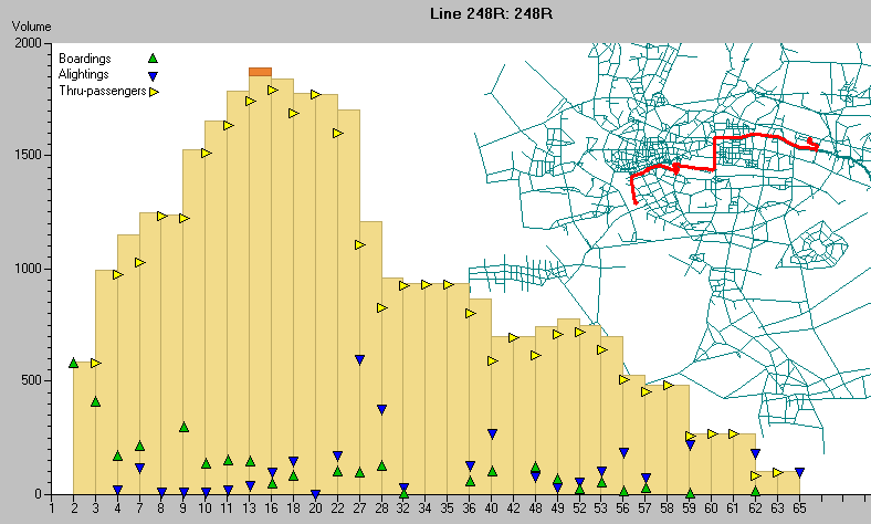
Figure 6.20 illustrates the same idea graphically. The link between Stop 13 and Stop 16 carries the heaviest load, so it is the critical link, and the maximum load on this critical link is about 1,800 passengers per hour per direction (or PPHPD). The maximum load on the critical link is of primary interest to BRT system planners, as it is used for making many crucial design and service planning decisions. The duration of one hour is considered the appropriate measure of peak duration (shorter measurements have considerable oscillation). In the formulas that follow, this peak load is called the “maximum hourly load on the critical link” (MaxLoad). Identifying this location and this load is paramount in any service planning exercise as it is the load at this point that will determine the fleet needed and the appropriate vehicle size. The expressions corridor maximum load and eventually system maximum load also refer to this measurement.
The “load factor” is the percentage of a vehicle’s total capacity that is actually occupied. For example, if a vehicle has a maximum capacity of 160 customers and 128 customers in a segment of a trip, then the load factor is 80 percent (128 divided by 160) on that given segment. The total load factor of the system would account for the average load for all services throughout the system (this average could be weighted by segment extension or time vehicles need to cross it), and it is used to show the efficiency with which the system’s vehicles are used. When the term load factor is used without further qualification, it refers to the design load factor—that is, the planned average load factor to happen on the busiest segment of the service, or the critical link, when the system is implemented as discussed in the following paragraphs.
The actual load factors of any BRT system are determined by the frequency of the vehicles, the capacity of the vehicles, and the demand. In a service plan, the load factor is easily altered by changing the frequency of the services, changing the vehicle size, or changing the routes of competing services. Designing services using a lower load factor than the real capacity of the vehicle is recommended.
While systems with high load factors tend to be more profitable, generally it is not advisable to plan to operate at a load factor of 100 percent. If designing for 100 percent load, 50 percent or more of the vehicles will be overcrowded, because the distribution of customers will never be uniform from vehicle to vehicle, but will likely be some variation within 10 to 20 percent of the design load factor. Even if the vehicles were at capacity and not overcrowded, the conditions in the vehicle will be uncomfortable to customers, as well as create negative consequences for operations. At 100 percent capacity, small system delays or inefficiencies, especially with boarding and alighting, can lead to severe overcrowding conditions.
The desired load factor may vary between peak and nonpeak periods. In Bogotá’s TransMilenio system, typical load factors are 80 percent for peak periods and 70 percent for nonpeak periods. However, as ridership levels increase in Bogotá, overcrowding becomes an increasing concern.
The load factor is unlikely to be uniform for the entirety of a route. Designing services that maintain high load factors for as much of the route as possible will tend to improve system performance and efficiency, including its financial performance.
A system’s capacity is considered to be met when the load factor reaches 100 percent at the maximum load on the critical link. Systems can also sometimes operate at a load factor exceeding 100 percent, but not by much, and such a system would be considered to be operating at “above capacity.” BRT system capacity is generally measured by the peak PPHPD. This measurement would be taken at the point of the maximum load on the critical link.
TransMilenio has a capacity of about 36,000 PPHPD based on its service plan, but its peak PPHPD has been counted as over 40,000. Such a level implies that customers are more closely packed than the maximum recommended levels. This situation is sometimes known as the “crush capacity.” While such extreme capacities can be expected in some unusual circumstances (e.g., immediately after special events such as sporting events or concerts), it is not desirable to regularly overcrowd vehicles.
6.3.9Service Frequency and Headways
The service frequency refers to the number of times a specific service is offered during a given time interval. Normally, frequency is expressed per hour, but service frequencies can also be expressed for any time interval, such as: “ten trips per day” or “twenty trips per three-hour peak period,” or even “a quarter of a trip per minute.” As with everything else in BRT service planning, frequency of service (existing or planned) changes throughout the day, but the sizing of the system should be based on the frequency during the peak hour. So, if no further mention is made, frequency means “the number of services provided in one hour, during the peak.”
The time between two vehicles offering a service, which conveys exactly the same information as frequency, is known as the “headway.” Headways can be expressed as, for example: “one trip every two hours” or as “one trip every ninety minutes” or “one trip every thirty seconds.” The characteristic of headway measuring is that time is referenced to one bus trip.
Based on the concept definitions, the below equations are always true (mathematical identities).
Eq. 6.1:
\[ \text{Freq} = {1 \over \text{hdwy}} \Leftrightarrow \text{hdwy} = {1 \over \text{Freq}} \]
Where:
- \(\text{Freq}\): Service frequency; that is number of times a specific service is offered during a given time interval;
- \(\text{hdwy}\): Service headway, that is time between two vehicles offering a service.
The service headway is the inverse of the frequency, but beware of units used for each one; for example: four buses per hour implies a headway of ¼ of hour, i.e., a headway of fifteen minutes. So the service headway in minutes is calculated as sixty divided by the frequency in hours and the frequency (in hours) is calculated as sixty divided by the headway in minutes.
The “minimum frequency” is the frequency that is needed to provide enough capacity to satisfy the existing demand without the average peak hour bus having a load factor above a policy-determined norm, usually 85 percent.
When planning services, if the vehicle size has already been determined, and an acceptable maximum load factor has been determined (normally 85 percent), then the minimum frequency can be determined based on the following formula:
Eq. 6.2:
\[ \text{Freq} = {\text{MaxLoad} \over {V_\text{Size} * \text{LoadFactor}}} \]
Where:
- \(\text{Freq}\): Service frequency; the number of times a specific service is offered during a given time interval;
- \(\text{MaxLoad}\): Maximum hourly load on the critical link;
- \(V_\text{Size}\): Vehicle capacity;
- \(\text{LoadFactor}\): Percentage of a vehicle’s total capacity that is actually occupied.
For example, if the bus specification has already been determined to have a capacity of 150 customers per vehicle, and the maximum hourly load on the critical link is 3,000, and the maximum acceptable load factor is 85 percent, or if:
\( \text{MaxLoad} = 2550 \);
\[ \text V_\text{Size} = 150; \]
\[ \text{LoadFactor} = 85 \% \]
Then:
\[ F = {2550 \over {150 \times 0.85} } = 20 \]
And if \(F = 20\), then the headway is \( {60 \text{(minutes)} \over {20}} = 3\text{(minutes)} \)
In general, it is desirable to provide frequent services in order to reduce customer waiting times. At headways of ten minutes or longer, customers will no longer have confidence that they can just show up at the station at any time and a bus will come in a reasonable period of time. With headways longer than 10 minutes, customers tend to view the system as a timetable service, which leads to loss of ridership. In Mexibus corridor III, illegal services operating parallel to the corridor serve most of the demand in off-peak hours.
In low demand systems where authorities want to promote increased public transport ridership, they sometimes set frequency based on a policy decision rather than on the minimum frequency. As very low demand routes are quite common in the developed world, it is often the case that frequency is set as a matter of policy rather than as a function of capacity. Services operating at frequencies higher than can be justified by the demand, however, are likely to contribute to operating deficits.
On a BRT system, a corridor with relatively high frequency should have been chosen, so the chances are that frequencies will rarely drop below six in any case. But what appears as high frequency in mixed traffic appears as low frequency on a busway. A five-minute frequency in mixed traffic is very high; on a busway, it is comparatively low. A busway with a headway of five minutes will appear empty most of the time to motorists sitting in traffic congestion. The lower the frequency, the greater the likelihood that motorists will complain that the road is being underutilized. Such complaints can ultimately undermine political support for future busways. In Quito, pressure from motorist organizations led the national police to open up exclusive busway corridors to mixed traffic for a period of time in 2006. This was also the case in León, Mexico in 2008. This conversion occurred despite the fact that each busway lane was moving three to four times the volume of customers as a mixed traffic lane. Nevertheless, the perception of an empty busway next to heavily congested mixed-traffic lanes can create political difficulties. A similar political battle has been fought over the BRT corridor in Indore, India.
On the other hand, if headways are very low, and frequency is very high, congestion at the station and service irregularity become a risk. Figure 6.23 illustrates the relationship between service frequency and congestion.
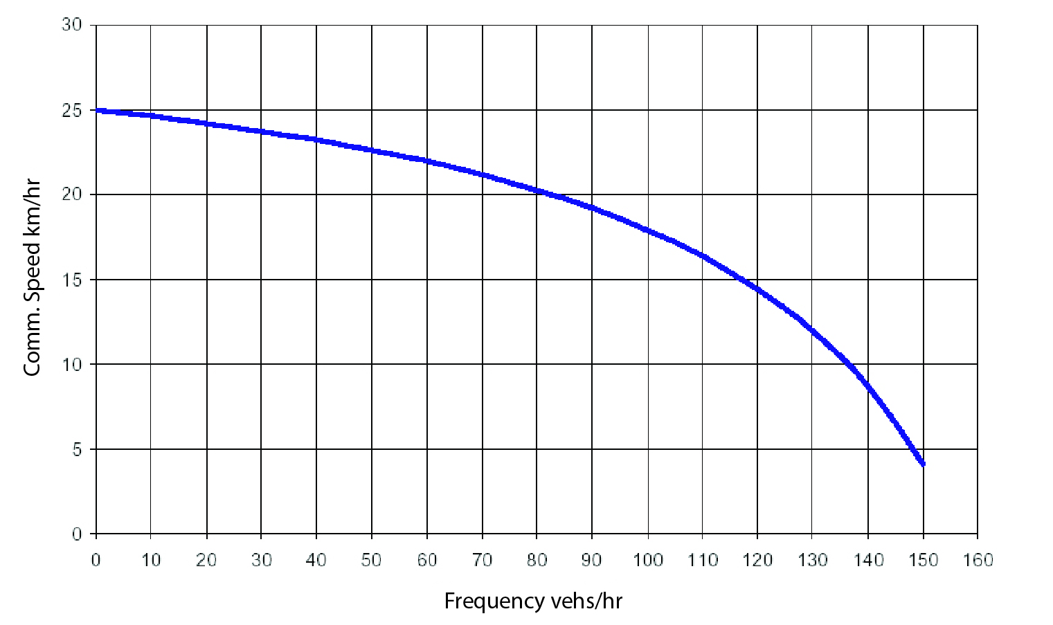
Service irregularity (bus bunching) is an even greater risk with higher frequency. For these reasons, it is usually advisable to split a service into two distinct services (for example, one limited and one express) if the frequency rises above 30 vehicles per hour.
6.3.10Dwell Time
One of the main aims of BRT system design and service planning is to reduce the delay caused by vehicles slowing down to stop at stations, allowing the customers to board and alight, and then to accelerate to a free-flow speed. The entirety of this delay is known as “total dwell time,” or Td, in this chapter’s equations.
The dwell time consists of two separate types of delay: “fixed dwell time” (\(T_0\)) and “variable dwell time.” In BRT system planning, it is critical to keep these two causes of delay distinct, because different decisions will affect different types of dwell time. Fixed dwell time, also called “dead time,” is the time consumed by a vehicle slowing down on approaching a station, opening its doors (and after a variable dwell time for boarding and alighting), closing its doors, and then regaining free-flow speed. This delay is called fixed dwell time because it does not vary with the number of customers boarding and alighting at each stop, and it does not vary much between stops in a system. The only way to reduce fixed dwell time is to remove stopping at particular stations in the service design, by offering express or limited stop services or eliminating the stop from the system.
In some countries, it is more typical to model fixed dwell time as only the time at the station when a bus is opening and closing its doors, and the time consumed accelerating and decelerating on the approach to the stop is modeled as a reduction in the link speed between station stops. It is important to keep in mind that this guide, when it talks of fixed dwell time, refers to both.
Variable dwell time consists of customer boarding time (\(T_b\)) and alighting time (\(T_a\)). Because it varies with the number of customers boarding and alighting at a given station, it is called “variable dwell time,” (\( T_b + T_a\) or \(max(T_a, T_b)\) depending on the vehicle/system configuration).
Many key elements of BRT that are recognized by The BRT Standard are measures that will tend to reduce variable dwell time, such as:
- Number of vehicle doorways;
- Width of vehicle doorways;
- Level boarding;
- Fare collection outside the vehicle.
BRT systems are able to operate metro-like service in large part due to the ability to reduce dwell time per customer from an average of five or six seconds per passenger for a typical bus service to only 0.3 seconds per customer on a Gold Standard BRT.
6.3.11Renovation Factor
The renovation factor (\(\text{Ren}\)) is total demand of a bus route divided by the load on the critical link of that route (note that operators customarily use the vehicle capacity instead of load on the critical link). It is the multiplier used to convert the number of customers that one would observe travelling on a route at the critical link (for example, in a vehicle occupancy survey) into the total number of customers on the route. Higher renovation factors are seen when there are many short trips along the line; corridors with very high renovation factor rates are more profitable because the same number of total paying customers is handled with fewer vehicles. For example, the Insurgentes corridor in Mexico City has a recorded renovation factor of five, which means that there are five times more people getting on and off the vehicle as there are people on the vehicle at the most loaded time.
Corridors with very high renovation factors meet higher demand more easily than corridors with low renovation factors, simply because more people are getting on and off vehicles along the corridor after shorter rides, so more people can be served.
Eq. 6.3:
\[\text{Ren}_\text{route} = {D_\text{route} \over \text{MaxLoad}_\text{route}}\]
Where:
- \(\text{Ren}_\text{route}\): Renovation factor of a route;
- \(D_\text{route}\): Route demand (in passengers);
- \(\text{MaxLoad}_\text{route}\): Route demand on the critical link.
6.3.12Irregularity Index (Irr)
The irregularity index is a number that expresses the reliability of actual headways against scheduled headways. An irregularity index of one means that the vehicles are arriving at completely random times, and an irregularity index of zero means that vehicles are arriving precisely when they are scheduled. It is measured as:
Eq. 6.4:
\[ \text{Irr} = {\text{Variance of the headway} \over {\text{Scheduled headway}} ^2 } \]
Where:
- \(\text{Irr}\): Irregularity index, the measure of the variance between the actual headways and the scheduled headways;
- \(\text{Variance of the headway}\): Amount that the headways are spread out;
- \(\text{Scheduled}_text{headway}\): Average waiting time between vehicles.
Variance of the headway is statistically defined as the expected value of the squared deviation from the mean headway. When calculating it from a sample it would be equal to the sum of the square of the differences between each observed headway and the average headway divided by the number of observations minus one, given by:
Eq. 6.5:
\[V_\text{hdwy} = {\sum_{i=1}^{N_\text{obs}} (\text{hdwy}_i - \text{hdwy}_\text{average}) ^ 2 \over {N_\text{obs} - 1}} \]
Where:
- \(V_\text{hdwy}\): Variance of the headway, expected value of the squared deviation from the mean headway;
- \(N_\text{obs}\): Number of observed headways;
- \(\text{hdwy}_i\): Observed headway for “i”;
- \(\text{hdwy}_\text{average}\): Average headway, average waiting time between vehicles = scheduled headway.
The average headway will generally be equal to the scheduled headway, unless fewer trips than scheduled regularly occur. Consider the extreme case where we should have one bus every twenty minutes every hour during ten hours, which would be thirty buses throughout the day (or three buses per hour for ten hours), and imagine that the first bus was on time and the other twenty-nine arrive one after another in the last half hour of the tenth hour. The headway of the first bus would be 571 minutes and the other 29 would be 1 minute, so on average the headway would still be 20 minutes per bus (600 minutes divided by 30 buses). Without an operational control system, empirical observation indicates that under many conditions, the irregularity index is around 0.3.
6.3.13Cycle Time-Related Concepts: Cycle Time (TC) and Maximum Demand Load per Cycle Time (MaxLoadperCycle)
Assuming that a vehicle will keep repeating a service (in both directions, or as a circular route), cycle time is the amount of time that it takes for a bus to travel the entire length of its route, in both directions, and be ready to begin a second circuit, including any time waiting and reversing direction at the end points. It is extremely important to know the cycle time per route for service planning. If a cycle time is short, the same bus can rapidly come back to the beginning of the route and take a second load of customers. If the cycle time is long, additional buses will be needed. Knowing the cycle time is therefore necessary for determining the required fleet.
When proposing an initial service plan, one should already have the existing route travel times in mixed traffic. In order to estimate the cycle time for the proposed routes, one must replace the travel time inside the BRT structure assuming a typical speed (say 20 kph if the corridor is in a dense downtown area, or 29 kph if it is on a limited-access high-speed arterial with few intersections). In the next chapter, methods of calculating more refined projected speeds will be presented, but for this chapter, these baseline speeds will be assumed for inside the BRT trunk operations.
It should be noted that drivers must have some rest time at the end of the route; in short routes this can be done once per cycle. Even if it would be possible to reduce the time to turn the vehicle by changing drivers, the practice is to have the driver always using the same vehicle, which eases operations management and fleet maintenance as well as improving the quality of driving.
Once the cycle time is estimated for each planned service, it is possible to estimate the Maximum Demand Load per Cycle Time (MaxLoadperCycle). This is the number of customers that are likely to accumulate over the course of the cycle time expecting to cross the critical link of the route. In other words, how many customers will accumulate for a specific route at the critical link over a time period equal to the cycle time? This figure, which can be calculated from the surveys of existing routes, is critical in several calculations in service planning. This figure is basically the same thing as the number of customer places that need to be serviced with vehicles, and is sometimes identified as “passenger places served.” It can be thought of as the size of the vehicle that would be needed if only one vehicle were used to service the peak hour demand.
For planning purposes, it is critical to know the peak load demand on a typical day over the course of a single cycle time (also during the peak period). If demand is reasonably constant throughout the day, and one can assume that hourly MaxLoad is constant, then MaxLoadperCycle would be estimated by:
Eq. 6.6a:
\[ \text{MaxLoadperCycle} = \text{MaxLoad} *\text{TC} \]
Where:
- \( \text{MaxLoadperCycle}\): Maximum demand load per cycle time;
- \( \text{MaxLoad}\): Maximum hourly load on the critical link;
- \( \text{TC}\): Cycle time in hours.
However, demand is rarely constant before and after the peak hour, nor even during the peak hour. If demand is at its peak, then the maximum demand load per cycle time will appear higher for an increment of time shorter than an hour than if it is averaged over an hour. For a cycle time longer than an hour, the maximum demand load for the cycle time will appear to be lower than for the peak hour because it is being averaged over a longer period of time during which the demand has already fallen. The more demand is peaked, the greater the distortion.
Therefore, to be more accurate, one has to apply a correction factor:
- Increases demand if the cycle time is shorter than one hour;
- Decreases demand if the cycle time is longer than one hour.
One way to apply such a correction is using the formula below:
Eq. 6.6b with “peak hour to cycle correction factor” (PHtoCC):
\[ \text{MaxLoadperCycle} = \text{MaxLoad} * TC * [ 1 - \text{PHtoCC} * (\text{TC} -1) ] \]
Where:
\(\text{PHtoCC}\): Nonnegative correction factor, the calibration of which is based on survey data, is discussed in Box 6.2. The usual value is near 0.1;
- If \(\text{TC}\) is larger than one hour: correction \( 1 - \text{PHtoCC} * (\text{TC} -1) \) will result smaller than one;
- If \(\text{TC}\) is smaller than one hour: correction \( 1 - \text{PHtoCC} * (\text{TC} -1) \) will result larger than one;
- If \(\text{TC}\) is equal one hour: correction \( 1 - \text{PHtoCC} * (\text{TC} -1) \) will result in one;
- If \(\text{PHtoCC}\) is equal zero, there will be no correction, and the formula is equal to the previous formula.
6.3.14Waiting Time (Twait) and Waiting Time Cost (Costwait)
Throughout this chapter it will be necessary to compare the relative costs and benefits of different service planning scenarios. One of the most important costs to consider in service planning is the cost of time spent waiting by customers.
Assuming customers arrive randomly at a bus stop, the average waiting time for a customer is only half of the observed headway of the route. Hence, the wait time per customer is the headway multiplied by 0.5, plus a little extra if there is irregularity in the actual headways from scheduled service (Irr). The equation below expresses this, replacing headway with frequency (its inverse value).
Eq. 6.7:
\[ T_\text{wait}= 0.5 * (1 + \text{Irr}_\text{route}) * \text{hdwy} = {0.5 * (1 + \text{Irr}_\text{route}) \over \text{Freq}}\]
Where:
- \(T_\text{wait}\): Time spent waiting per customer;
- \(\text{Irr}\): Irregularity index; measure of the variance between the actual headways and the scheduled headways (usually near 0.3, see Section 6.3.9);
- \(\text{hdwy}\): Route Headway;
- \(\text{Freq}\): Route Frequency.
The cost of waiting (\(\text{Cost}_\text{wait}\)) is defined as the amount an average customer would spend to avoid waiting for a vehicle, it is measured in currency per unit of time—for example: “5 Rp. per minute” and “6 US$ per hour”—and is calculated as a fraction of customer income. Costwait varies depending on a city’s income and proclivity, but typically, people value their time at about one-third of the average wage rate, and are willing to pay twice as much to avoid waiting for a vehicle (i.e., 66 percent of the average user wage).
Customers do not like to wait for a vehicle. If the demand of a given route proposed on a service plan is known (initially it can be approximated by using the demand on a similar existing route), the total waiting cost caused by a route is the sum of the cost of waiting time imposed on all its customers (assuming for now that this is captive demand), then multiplied by their value of waiting time:
Eq. 6.8a:
\[\text{WaitCost}_\text{route} = \text{D}_\text{route} * \text{Cost}_\text{wait}*\text{T}_\text{wait}\]
Where:
- \(\text{WaitCost}_\text{Route}\): Total waiting time cost for the users of the route (in US$);
- \(\text{D}_\text{route}\): Route demand (in passengers);
- \( \text{Cost}_\text{wait}\): Average user waiting cost ($/time);
- \(\text{T}_\text{wait}\): Average user waiting time (time/passenger).
This is the total cost of waiting faced by all the customers on a particular route during the peak hour. The average value of waiting as defined is the same all day.
The \(\text{D}_\text{route}\) formula for estimating the cost of waiting on the route would be more usefully expressed as a function of the maximum load on the critical link and of the route frequency because normally one has a sense of where the most crowded link on a public transport route is, and one can count the number of buses per hour, and estimate their occupancy from vehicle frequency and occupancy counts. One might know the total ridership on one route, but not all of them, so one can estimate the total demand on the corridor for all the routes by using an average renovation rate on the corridor. To do this, the formula can be rewritten as follows:
Eq. 6.3 can be rewritten:
\[\text{Ren}_\text{route} = {{D}_\text{route} \over \text{MaxLoad}_\text{route}} \Leftrightarrow \text{D}_\text{route} = \text{MaxLoad}_\text{route} * \text{Ren}_\text{route}\]
This is simply true by definition. Remember that the renovation rate of the route is by definition the total demand on the route divided by the maximum load on the critical link, or that the demand on the route is a function of the maximum load on the critical link multiplied by the renovation rate.
We can then replace Droute and Twait from Equation 6.2 and Equation 6.6 in Equation 6.7, so that we have:
Eq. 6.8b:
\[ \text{WaitCost}_\text{route} = \text{D}_\text{route} * \text{Cost}_\text{wait} * \text{T}_\text{wait}\]
\[ \text{WaitCost}_\text{route}= {\text{MaxLoad}_\text{route} *\text{Ren}_\text{route} * \text{Cost}_\text{wait} * 0.5 * (1 + \text{Irr}_\text{route}) \over \text{Freq}_\text{route} }\]
Where:
- \( \text{WaitCost}_\text{route}\) = Total waiting time cost generated to the route users (now in $/hour because instead of giving Droute absolute value in passengers, it is being given in passengers/hour);
- \( \text{Ren}_\text{route}\): Renovation factor of a route;
- \( \text{MaxLoadroute}\): Route demand on the critical link (now in passengers/hour or “pax” per hour);
- \( \text{Cost}_\text{wait}\): Average user waiting cost ($/time);
- \( \text{Irr}\text{route}\): Irregularity index of the route; measure of the variance between the actual headways and the scheduled headways (usually near 0.3, see Section 6.3.9);
- \(\text{Freq}_\text{route}\): Frequency of the route (vehicles/time).
6.3.15Vehicle Operating Cost
Often, in service planning, the costs of waiting for customers, which is a function of the frequency and regularity of service, will need to be balanced against the cost of operating more vehicles. As the costs of waiting have been calculated for the peak hour above, to make a valid comparison the vehicle operating costs should also be derived per hour. The formulas below can be used to estimate cost per bus (Costbus) and the fixed cost per bus (BusFixedCost or Costbus-fixed). Vehicle operating cost per hour is simply the total cost of operating a vehicle divided by the number of hours a vehicle is in service.
The fixed operating cost of a vehicle is the part of the vehicle operating cost that does not depend of the number of customers carried nor the size of the vehicle. It can be thought of as the cost operators would incur if they put a second vehicle in operation, but that vehicle never opened its doors and always ran empty. It is mostly the cost of the driver, but also the minimum cost in terms of fuel and maintenance that any vehicle would incur regardless of its size. This figure is important to calculating the optimal fleet size. This part of the cost exists whether one is expressing the costs per route, per vehicle, per vehicle hour, or per vehicle kilometer.
To calculate the total fixed operational cost for a route, simply multiply the fixed operating cost per vehicle times the total fleet needed to service that route, or:
Eq. 6.9:
\[\text{RouteFixedCost} = \text{BusFixedCost} * \text{Fleet}_\text{route} \]
Where:
- \( \text{RouteFixedCost}\): Total fixed operational cost for the route;
- \( \text{BusFixedCost}\): Fixed operating costs per vehicle;
- \( \text{Fleet}_\text{route}\): Number of buses needed to operate the route.
Total operating cost per vehicle goes down when a stop is removed, as the speed of the vehicles increases. As such, total vehicle operating costs are used in Section 6.7 on limited stop services. When optimizing the size of the vehicle, as in Section 6.4, as well as when comparing direct against trunk-and-feeder services in Section 6.6, it is only the fixed costs of vehicle operation that need to be known because it will be necessary to determine the benefits of using larger vehicles, and what is eliminated by using larger vehicles is the cost of the vehicle that does not go up proportionally with the size of the vehicle. It can be calculated by simply calculating the hourly operating cost of the smallest vehicle in the fleet. Typically, this ranges from US$10 to US$100 per bus hour. It will vary from country to country, but not much from city to city, so it only needs to be calculated once in a given city or country. The BusFixedCosts value consists of a list of average costs per vehicle. Fixed maintenance and fuel costs, which are likely to vary somewhat by vehicle size, should be calculated for the smallest vehicle being considered, and any additional costs for these will be included in variable costs. In most of this chapter one should use a common \( \text{Cost}_\text{bus-fixed} \) value of US$30 per vehicle hour.