6.6Direct Services, Trunk-and-Feeder Services, or Hybrids
Paths cross all the time in this world of ours, sometimes in the strangest places.Stephen King, writer, 1947–
When designing new services for a BRT system, the project team must decide which preexisting bus routes that continue beyond the BRT corridor should be incorporated into the new BRT service plan as “direct” services that enter and exit the BRT corridor, and which should be split into trunk routes operating inside the BRT infrastructure and feeder routes operating in mixed traffic and “feeding” the trunk stations. Whether and when to do this has been the subject of debate among BRT service planners. This section provides some basic guidance on how to make this determination in specific cases.
In general, most customers would prefer to take a bus directly from where their trip begins to where it ends. New BRT infrastructure on one corridor is not going to fundamentally change people’s trip origins and destinations in the short term. The new BRT infrastructure is likely to be built on a corridor with multiple preexisting public transport services that not only run up and down the corridor, but also continue beyond the corridor. Chances are that many people will not have destinations within walking distance of the new BRT stations, so if the preexisting services are discontinued, and only one BRT trunk service is running up and down the BRT infrastructure, many customers will be forced to use feeder services and transfer to trunk in stations along the corridor or at larger terminals. In the worst case, this transfer delay may be greater than the time benefit of using the BRT system.
The most important differences in the costs and benefits of direct services versus trunk-and-feeder services are as follows (listed here and described in detail below):
- Fleet requirements: When demand is peaked, as is generally the case, more fleet is required for trunk-and-feeder services than for direct services. When demand is flat, fleet requirements are basically equivalent;
- Vehicle sizes: When the trunk portion of the route is longer than the feeder portion, and many routes share the trunk corridor, larger vehicles can be used on the trunk routes, providing a cost savings for trunk-and-feeder services over direct services;
Transfer costs: The greater the delay caused by the introduction of the new transfer, the greater the additional cost of trunk-and-feeder services, including:
- Running time;
- Boarding and alighting delay;
- Suboptimal terminal location;
- Suboptimal terminal design on walking time;
- Land acquisition and terminal construction costs.
- Station saturation: The greater the risk of trunk corridor station platform saturation, the greater the benefit of trunk-and-feeder services.
This section systematically analyzes these key factors. Factors that did not vary significantly between trunk-and-feeder and direct service modes were not further considered. For instance, while some claim to prefer trunk-and-feeder systems to reduce irregularity of service inside the BRT trunk corridor, there is little empirical evidence to suggest any significant overall system-wide benefit of this. Having irregular arrivals of feeder buses at transfer terminals where conditions can become severely overcrowded, as frequently happens in Bogotá’s TransMilenio, is as problematic as having irregular direct services with a dispersed impact along the BRT trunk corridor.
The following sections provide some formulas based on the above criteria that should assist in making decisions about which bus routes to retain as direct services and which to cut into trunk-and-feeder services. As there are many variables to consider, alternatives should ideally be tested using a public transport demand model, and this should be complemented by an analysis of saturation and delays of each proposal at critical points such as at stations and signals.
6.6.1Fleet Requirements for Direct Versus Trunk-and-Feeder Services
All other things being equal, trunk-and-feeder systems tend to require larger fleets than direct service systems, and the amount of extra fleet needed will vary based in large part on the degree to which the demand is concentrated in peak periods. This subsection explains the reasons for this effect, and uses the method of calculating fleet requirements in specific conditions.
As was discussed above in Section 6.4, the fleet size per route is generally determined by the fleet required to satisfy the maximum load that accumulates on the critical link during the course of the route cycle time during the peak period (Eq. 6.18: \( \text{Fleet}_\text{route} = {\text{MaxLoad}_\text{route} \over \text{VSize} * \text{LoadFactor}} \) ). Below, a series of scenarios illustrate the point, each with more complicated assumptions.
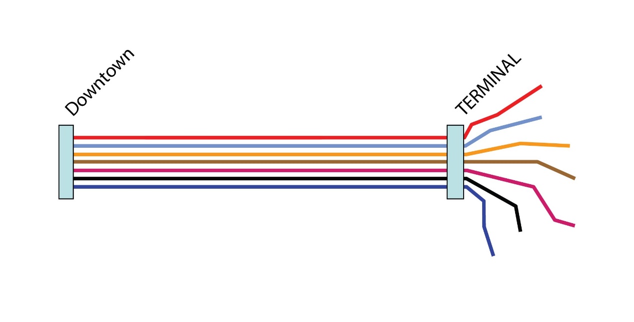
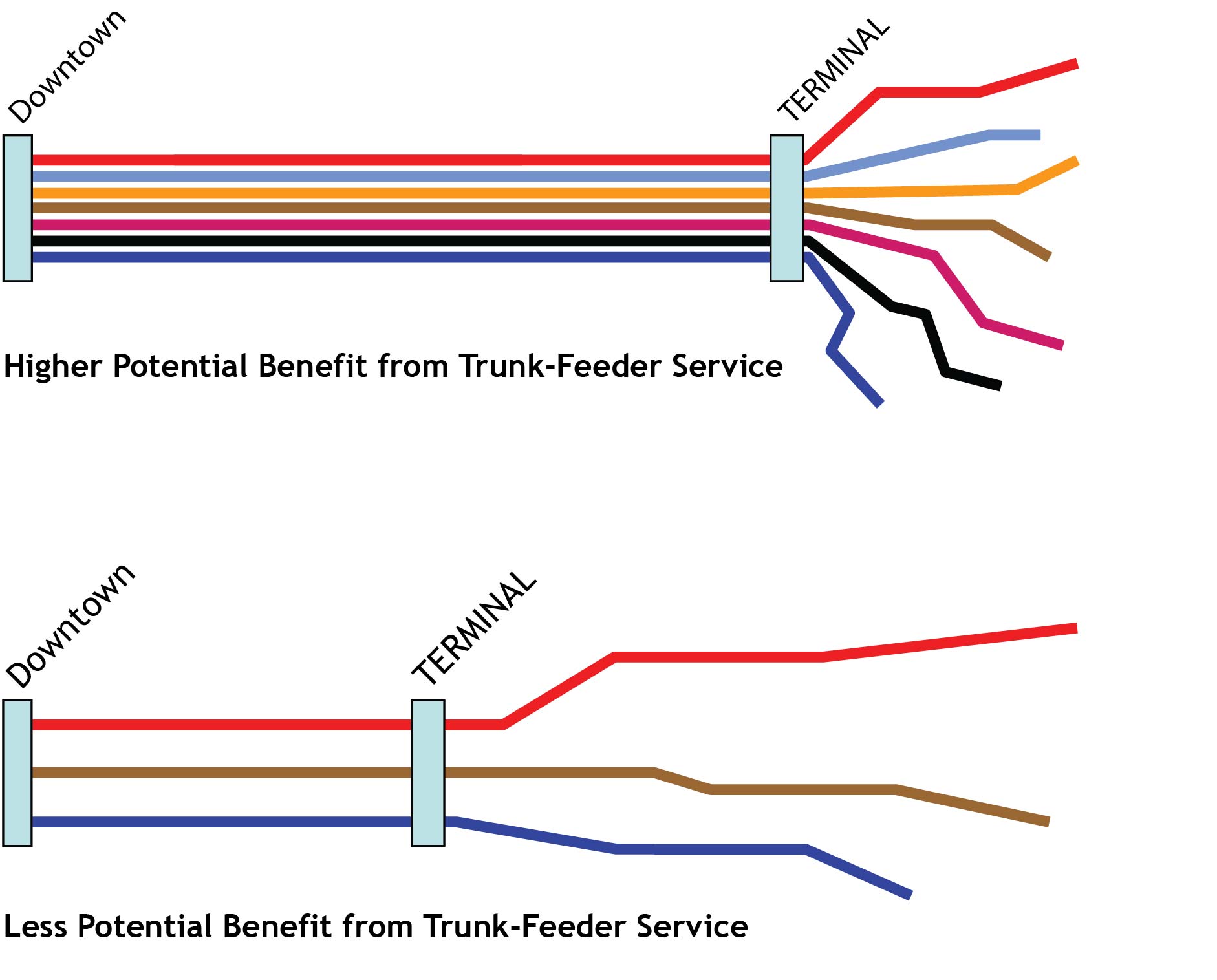
First, the fleet requirements for direct services with uniform demand throughout the day will be discussed. Then, calculating the fleet if demand varies between peak and off peak will be reviewed. Finally, some of the direct routes are split into trunk-and-feeder routes using the principles from the previous scenarios and fleet needs are compared between direct services and trunk-and-feeder services. In order to do this, one should have a BRT corridor with services that look like the diagram in Figure 6.41.
We make the following additional assumptions:
- A One should have already determined that the bus capacity (VSize), for the examples being considered have a design load factor of 85 percent, so in these examples the bus capacity is 60 passengers, though the real BRT vehicle capacity is 70 passengers;
- B All the bus routes operate on full BRT infrastructure between Downtown and the Terminal (as in diagram Figure 6.41), and all services operate in mixed traffic beyond the Terminal;
- C There is no overlap of routes until they reach the common point, Terminal;
- D The critical link with the maximum aggregate load (i.e., the load for all routes combined) occurs somewhere near the Terminal and continues at a similar level to Downtown;
- E The peak hour, in the cases where it exists, occurs earlier in the day on the link before the Terminal and later between the Terminal and Downtown.
6.6.1.1Comparative Fleet Advantages under Flat Demand with Uniform Routes
In this situation, two service patterns are compared:
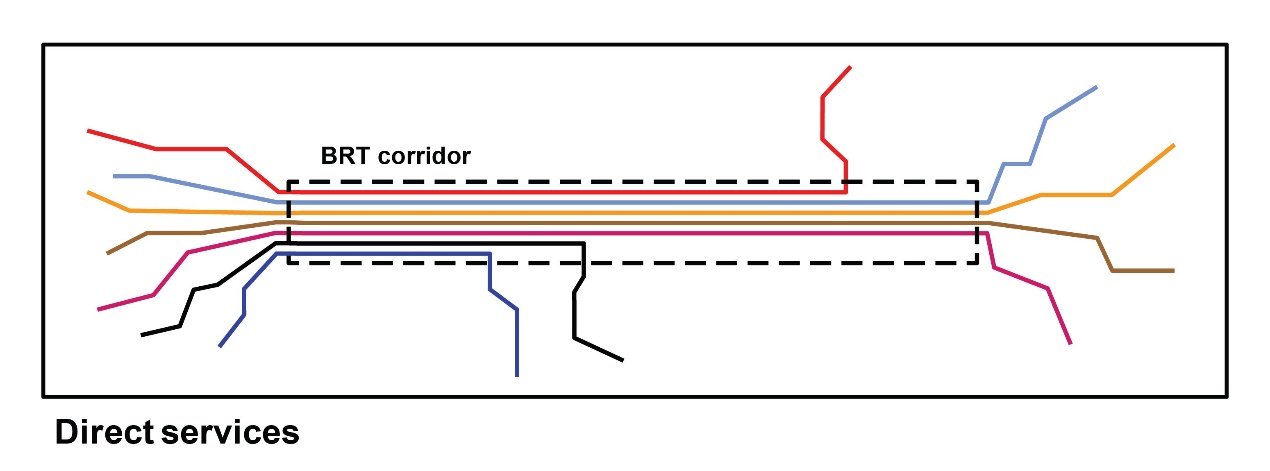
- Direct Services: A service pattern where multiple bus routes run in mixed traffic on local streets and then continue onto the BRT corridor (Figure 6.42).
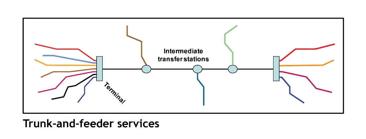
- Trunk-and-Feeder Services: A service pattern where multiple bus routes run in mixed traffic on local streets and terminate at a single terminal. Another bus route with higher frequency operates up and down the BRT corridor, and customers travelling between one and the other must transfer.
When designing a BRT system, normally one could assume a reasonable BRT speed to be the equivalent of the speed of a vehicle operating during off-peak conditions, or one could assume a Gold Standard BRT system speed will be roughly 20 kph in a downtown area and about 25 kph on a major urban arterial. For this analysis, the cycle time (TC) of a direct service route will be the time spent on the trunk (at off-peak speeds) plus the time spent on the mixed traffic portion of the route at existing peak-hour mixed traffic speeds. For the trunk-and-feeder alternative, the TC of the trunk route will just be the time spent on the trunk portion of the route at off-peak speeds, and the feeder portion of the route will be the feeder portion of the route at existing peak-hour mixed traffic speeds. Therefore, one should define three types of TCs:
Eq. 6.38
\[ TC_\text{Trunk}=(L_\text{Trunk}*V_\text{Trunk Outbound})+(L_\text{Trunk}*V_\text{Trunk Inbound}) \]
Where:
- \( TC_\text{Trunk} \): Cycle time in hours for a vehicle to complete one circuit of the trunk;
- \( L_\text{Trunk} \): Length of the trunk;
- \( V_\text{Trunk Outbound} \): Velocity on the outbound trunk;
- \( V_\text{Trunk Inbound} \): Velocity on the inbound trunk.
Eq. 6.39
\[ TC_\text{Feeders}=L_\text{Feeders}*V_\text{Feeders Outbound}+L_\text{Feeders}*V_\text{Feeders Inbound}\]
Where:
- \( TC_\text{Feeders} \): Cycle time in hours for a vehicle to complete one circuit of the feeders;
- \( L_\text{Feeders} \): Length of the feeders;
- \( V_\text{Feeders Outbound}\): Velocity on the outbound feeder;
- \( V_\text{Feeders Inbound}\): Velocity on the inbound feeder.
For our analysis, it is assumed that the cycle time for the trunk routes plus the cycle time for the feeder routes is as short as possible, being equivalent to the cycle time for the direct service routes or:
Eq. 6.40
\[ TC_\text{direct}=TC_\text{trunk}+TC_\text{feeder} \]
Where:
- \( TC_\text{Direct} \): Cycle time in hours for a vehicle to complete one circuit of the trunk-and-feeder services;
- \( TC_\text{Trunk} \): Cycle time in hours for a vehicle to complete one circuit of the trunk service;
- \( TC_\text{Feeder} \): Cycle time in hours for a vehicle to complete one circuit of the feeder service;
Under these conditions, the benefit of a direct service will be the difference in the fleet requirements between Service Plan A and Service Plan B:
Eq. 6.41
\[ \text{Fleet}_\text{benefit direct}=\text{Fleet}_\text{trunk}+\text{Fleet}_\text{feeder}–\text{Fleet}_\text{direct} \]
Where:
- \( \text{Fleet}_\text{benefit direct} \): Benefit of a direct service in terms of the fleet;
- \( \text{Fleet}_\text{trunk} \): Fleet requirement for the trunk service;
- \( \text{Fleet}_\text{feeder} \): Fleet requirement for the feeder service;
- \( \text{Fleet}_\text{direct} \): Fleet requirement for the direct service.
Recall Equation 6.18 from Section 6.4, which shows that the fleet size is determined by the maximum load of passengers that accumulates over the course of the cycle time for a given bus size.
Equation 6.18 applied:
\[ \text{Fleet}_\text{direct} = {\text{MaxLoadperCycle}_\text{direct} \over \text{VSize} * \text{LoadFactor}} \]
\[ \text{Fleet}_\text{trunk} = {\text{MaxLoadperCycle}_\text{trunk} \over \text{VSize} * \text{LoadFactor}} \]
\[ \text{Fleet}_\text{feeder} = {\text{MaxLoadperCycle}_\text{feeder} \over \text{VSize} * \text{LoadFactor}} \]
Where:
- \( \text{Fleet}_\text{trunk} \): Fleet requirement for the trunk service;
- \( \text{Fleet}_\text{Feeder} \): Fleet requirement for the feeder service;
- \( \text{Fleet}_\text{direct} \): Fleet requirement for the direct service.
- \( \text{MaxLoadperCycle}_\text{trunk} \): Maximum load on the trunk service for one cycle time;
- \( \text{MaxLoadperCycle}_\text{feeder} \): Maximum load on the feeder service for one cycle time;
- \( \text{MaxLoadperCycle}_\text{direct} \): Maximum load on the direct service for one cycle time;
- \( \text{VSize} \): Vehicle capacity;
- \( \text{LoadFactor}\): Design load factor (usually 0.85), which is the same for all routes.
The main assumption of this scenario, that the demand is uniform throughout the day, implies that the maximum load in the critical link (MaxLoad) is equal at any time. So the maximum load considered per cycle time (MaxLoadperCycle) for any given cycle time would be equal to the sum of two “maximum load per cycle” of smaller cycles times that add up to the same time, or, starting from Eq. 6.6a.
Eq. 6.6a
\[ \text{MaxLoadperCycle}=\text{MaxLoad}*TC \]
\[ \text{MaxLoadperCycle}_{T1}=\text{MaxLoad}*T1 \]
\[ \text{MaxLoadperCycle}_{T2}=\text{MaxLoad}*T2 \]
\[ \text{MaxLoadperCycle}_{T1+T2}=\text{MaxLoad}*(T1+T2) \]
Eq. 6.42
\[ \text{MaxLoadperCycle}_(T1+T2)= \text{MaxLoadperCycle}T1 + \text{MaxLoadperCycle}_T2 \]
Where:
- \( \text{MaxLoadperCycle}_(T1+T2) \): Maximum load considered for the sum of cycle times 1 and 2;
- \( \text{MaxLoadperCycle}_T1 \): Maximum load considered for cycle time 1;
- \( \text{MaxLoadperCycle}_T2 \): Maximum load considered for cycle time 2.
Therefore, as long as \( TC_\text{direct}=TC_\text{trunk}+TC_\text{feeder} \) the benefit of direct service is zero, as we show below:
\[ \text{Fleet}_\text{benefitdirect}=(\text{Fleet}_\text{trunk}+\text{Fleet}_\text{feeder})–\text{Fleet}_\text{direct} \]
\[ = ( {\text{MaxLoadperCycle}_\text{trunk} \over \text{VSize} * \text{LoadFactor}}+{\text{MaxLoadperCycle}_\text{feeder} \over \text{VSize} * \text{LoadFactor}}) - {\text{MaxLoadperCycle}_\text{direct} \over \text{VSize} * \text{LoadFactor}} \]
\[ = {\text{MaxLoadperCycle}_\text{trunk} + \text{MaxLoadperCycle}_\text{feeder} - \text{MaxLoadperCycle}_\text{direct} \over \text{VSize} * \text{LoadFactor}} \]
\[ = {\text{MaxLoadperCycle}_\text{trunk} + \text{MaxLoadperCycle}_\text{feeder} - \text{MaxLoadperCycle}_\text{trunk+feeder} \over \text{VSize} * \text{LoadFactor}} \]
\[ = {\text{MaxLoadperCycle}_\text{trunk} + \text{MaxLoadperCycle}_\text{feeder} - (\text{MaxLoadperCycle}_\text{trunk} + \text{MaxLoadperCycle}_\text{feeder} ) \over \text{VSize} * \text{LoadFactor}} \]
\[ = 0 \]
As an example we use a cycle time (TC) on the trunk of one hour, as well as a cycle time on the feeders in mixed traffic of one hour. So:
\[ TC_\text{trunk}=1 \text{hour} \]
\[ TC_\text{feeder}=1 \text{hour} \]
\[ TC_\text{direct}=2 \text{hour} \]
This example assumes that the optimal vehicle capacity was already determined (see previous introduction subsection) to be sixty passengers.
The \( \text{MaxLoadperCycle} \) for two hours is precisely double the maximum load for a cycle time of one hour, or:
\[ \text{MaxLoadperCycle}_\text{2 hours} = 2 * \text{MaxLoadperCycle}_\text{1 hour} \]
In this case, one should assume that \( \text{MaxLoad} = 225 \text{pax}/\text{hour} \), and one knows that demand is flat throughout the day, so the \( \text{PHtoCC} = 0 \), therefore:
\[ \text{MaxLoadperCycle}_\text{direct} = 225 * 2 = 450 \]
And the fleet required for the trunk-and-feeder scenario is:
\[ \text{Fleet}_\text{direct} = 450 \over 60 = 7.5 (ROUNDUP) = 8 \]
In the trunk-and-feeder scenario,
\[\text{MaxLoadperCycle}_\text{trunk} = \text{MaxLoadperCycle}_\text{feeder} = 225 *2 = 450 \]
\( \text{Fleet}_\text{trunk} = 225 \over 60 = 3.75 (ROUNDUP) = 4 \) \( \text{Fleet}_\text{feeder} = 225 \over 60 = 3.75 (ROUNDUP) = 4 \) \( \text{Fleet}_\text{direct benefit} = (4+4) - 8 =0 \)
In this case, the fleet needed for the direct service scenario is the same as the fleet needed for the trunk-and-feeder service option. If there were a rounding error, the trunk-and-feeder option may require a slightly larger fleet due to rounding, but the additional fleet is not that significant.
6.6.1.2Comparative Fleet Advantages under Peaked Demand with Uniform Routes
If the demand is peaked, but the routes remain uniform, the fleet requirements change, and direct services have a distinct advantage over trunk-and-feeder services. The advantage is proportional to double the peak hour to cycle correction factor (PHtoCC).
Remembering that and (Eq. 6.6b) the fleet benefit for using a direct route will be given by:
Eq. 6.43
\[ \text{Fleet}_\text{benefitdirect}=(\text{Fleet}_\text{trunk}+\text{Fleet}_\text{feeder})–\text{Fleet}_\text{direct} \]
\[ = {\text{MaxLoadperCycle}_\text{trunk} + \text{MaxLoadperCycle}_\text{feeder} - (\text{MaxLoadperCycle}_\text{trunk} + \text{MaxLoadperCycle}_\text{feeder} ) \over \text{VSize} * \text{LoadFactor}} \]
\[ = {\text{MaxLoad}*TC_\text{trunk} * [1 - \text{PHtoCC} * (\text{TC}_\text{trunk} -1) ] + \text{MaxLoad}*TC_\text{feeder} * [1 - \text{PHtoCC} * (\text{TC}_\text{feeder} -1) ] \over \text{VSize} * \text{LoadFactor}} \]
\[ - {\text{MaxLoad}*(TC_\text{trunk} + TC_\text{feeder}) * [1 - \text{PHtoCC} * ((TC_\text{trunk} + TC_\text{feeder}) -1) ] \over \text{VSize} * \text{LoadFactor}} \]
\[ = {\text{MaxLoad}*TC_\text{trunk} * [1 - \text{PHtoCC} * (\text{TC}_\text{trunk} -1) ] + \text{MaxLoad}*TC_\text{feeder} * [1 - \text{PHtoCC} * (\text{TC}_\text{feeder} -1) ] \over \text{VSize} * \text{LoadFactor}} \]
\( - {\text{MaxLoad}*TC_\text{trunk} * [1 - \text{PHtoCC} * ((TC_\text{trunk} + TC_\text{feeder}) -1) ] \over \text{VSize} * \text{LoadFactor}} \) \( - {\text{MaxLoad}*TC_\text{feeder} * [1 - \text{PHtoCC} * ((TC_\text{trunk} + TC_\text{feeder}) -1) ] \over \text{VSize} * \text{LoadFactor}} \)
\( = {\text{MaxLoad}*TC_\text{trunk} * \{[1 - \text{PHtoCC} * (\text{TC}_\text{trunk} -1) ] - [1 - \text{PHtoCC} * ((TC_\text{trunk} + TC_\text{feeder}) -1) ]\} \over \text{VSize} * \text{LoadFactor}} \) \( + {\text{MaxLoad}*TC_\text{feeder} * \{[1 - \text{PHtoCC} * (\text{TC}_\text{feeder} -1) ] - [1 - \text{PHtoCC} * ((TC_\text{trunk} + TC_\text{feeder}) -1) ]\} \over \text{VSize} * \text{LoadFactor}} \)
\( = {\text{MaxLoad}*TC_\text{trunk} * \{[1 - \text{PHtoCC} * \text{TC}_\text{trunk} + \text{PHtoCC} ] - [1 - \text{PHtoCC} * TC_\text{trunk} -\text{PHtoCC} * TC_\text{feeder} + \text{PHtoCC} ]\} \over \text{VSize} * \text{LoadFactor}} \) \( + {\text{MaxLoad}*TC_\text{feeder} * \{[1 - \text{PHtoCC} * \text{TC}_\text{feeder} + \text{PHtoCC} ] - [1 - \text{PHtoCC} * TC_\text{trunk} -\text{PHtoCC} * TC_\text{feeder} + \text{PHtoCC} ]\} \over \text{VSize} * \text{LoadFactor}} \)
\[ = {\text{MaxLoad}*TC_\text{trunk} * \{TC_\text{feeder} + \text{PHtoCC} \} \over \text{VSize} * \text{LoadFactor}} + {\text{MaxLoad}*TC_\text{feeder} * \{TC_\text{trunk} + \text{PHtoCC} \} \over \text{VSize} * \text{LoadFactor}} \]
\[ = 2* {\text{MaxLoad}*TC_\text{trunk} * TC_\text{feeder} * \text{PHtoCC} \over \text{VSize} * \text{LoadFactor}} \]
Where
\(\text{PHtoCC}\): Nonnegative correction factor, the calibration of which is based on survey data, is discussed in Box 6.2. The usual value is near 0.1;
- If \(\text{TC}\) is larger than one hour: correction \( 1 - \text{PHtoCC} * (\text{TC} -1) \) will result smaller than one;
- If \(\text{TC}\) is smaller than one hour: correction \( 1 - \text{PHtoCC} * (\text{TC} -1) \) will result larger than one;
- If \(\text{TC}\) is equal one hour: correction \( 1 - \text{PHtoCC} * (\text{TC} -1) \) will result in one;
- If \(\text{PHtoCC}\) is equal zero, there will be no correction, and the formula is equal to the previous formula.
- \( \text{MaxLoad}\): Maximum hourly load on the critical link;
- \( \text{TC}\): Cycle time in hours.
- \( TC_\text{Direct} \): Cycle time in hours for a vehicle to complete one circuit of the trunk-and-feeder services;
- \( TC_\text{Trunk} \): Cycle time in hours for a vehicle to complete one circuit of the trunk service;
- \( TC_\text{Feeder} \): Cycle time in hours for a vehicle to complete one circuit of the feeder service;
- \( Fleet_\text{trunk} \): Fleet requirement for the trunk service;
- \( VSize \): Vehicle capacity;
- \( LoadFactor\): Design load factor (usually 0.85), which is the same for all routes.
As an example, we keep the same assumptions from the previous case, but consider a peaked demand of 265 where the correction factor is given by 0.15 (see Box 6.2 How to determine correction factor from hour to cycle time (\(PHtoCC\)) based on load observations):
\( \text{MaxLoadperCycle}_\text{direct} \) \( = \text{MaxLoad} * (TC_\text{direct}*(1 - \text{PHtoCC} * (\text{TC}_\text{direct} -1))) \) \( = 265 * 2 * ( 1 -0.15 * 2 -1))) = 450 \)
\( \text{MaxLoadperCycle}_\text{feeder} = \text{ MaxLoadperCycle}_\text{trunk} \) \( = \text{MaxLoad} * (TC_\text{feeder}*(1 - \text{PHtoCC} * (\text{TC}_\text{feeder} -1))) \) \( = 265 * 1 * ( 1 -0.15 * 1 -1))) = 265 \)
In the case of the direct service option,
\[ \text{Fleet}_\text{direct} = {\text{MaxLoadperCycle}_\text{direct} \over \text{VSize} * \text{LoadFactor}} = {450 \over 60} = 7.5 (ROUNDUP) = 8 \]
In the case of the trunk-and-feeder option:
\[ \text{Fleet}_\text{trunk} = {\text{MaxLoadperCycle}_\text{trunk} \over \text{VSize} * \text{LoadFactor}} = {265 \over 60} = 4.417 (ROUNDUP) = 5 \]
\[ \text{Fleet}_\text{feeder} = {\text{MaxLoadperCycle}_\text{feeder} \over \text{VSize} * \text{LoadFactor}} = {265 \over 60 } = 4.417 (ROUNDUP) = 5 \]
So:
\[ \text{Fleet}_\text{directbenefit} = (\text{Fleet}_\text{trunk}+\text{Fleet}_\text{feeder})–\text{Fleet}_\text{direct} =(5+5) – 8 = 2 \text{vehicles} \]
We save two vehicles by using direct services over a trunk-and-feeder service plan on this route. One way to think about this is that the peak demand in the mixed traffic section of the routes occurs earlier in the day, so the same vehicles in a direct services service plan needed to serve the peak-hour demand on the mixed traffic “feeder” portion of the route can continue past the terminal and serve the peak-hour demand, occurring slightly later, on the trunk. With the trunk-and-feeder service plan, buses need to serve the peak demand on the feeder routes at close to the same time as on the trunk. So, while it is peak time for the feeders, the trunk vehicles are waiting, and then, as the peak demand shifts toward the trunk, some of the feeder vehicles will be unused. A direct services service plan therefore uses a smaller fleet because it optimizes the fleet by serving the demand as it moves through the corridor.
In this example, the benefit was evaluated for just one route. If one does the analysis for ten equivalent routes, and all have the same TC, the difference in fleet would be multiplied by ten, and the difference becomes significant.
6.6.2Vehicle Size Optimization Benefits for Trunk-and-Feeder versus Direct Services
The main advantage of a trunk-and-feeder service is that the demand on the feeder routes, which in isolation would be served by small vehicles with high operating costs per customer, can be combined on the trunk portion of the route, so that customers from multiple feeder routes can all use a much larger trunk vehicle. Because large vehicles at high occupancy levels have lower operating costs per customer than smaller vehicles, there is a benefit of lower vehicle operating costs with trunk-and-feeder services in appropriate conditions. This section identifies easy ways of spotting what those conditions are, to conclude the following:
The greater the number of routes being combined into a trunk route, and the greater the proportion of the total trip that is taken up by the trunk portion of the trip, the greater the benefit.
Applying the formulas presented before, the benefits of optimal fleet size can be compared under different service plan alternatives as applied to some typical conditions. In both scenarios simplified examples are first introduced to illustrate general principles, and then the general formulas are applied to more real-world situations.
6.6.2.1Vehicle size optimization with several similar feeder routes:
In this example, one looks at the benefits of trunk-and-feeder systems from using bigger vehicles on the trunk portion of the route for BRT projects where the following conditions apply:
- A All routes have similar demand;
- B All routes extend beyond the trunk corridor for a similar distance and at similar speeds, and all routes leave the trunk corridor at roughly the same place;
- C The peak-hour load (\(MaxLoad\)) for the trunk is similar to the peak-hour load for all of the combined feeders;
- D No transfer time is required to get from the feeder vehicle to the trunk vehicle, just waiting time;
- E No extra time is required for vehicles to pull off the BRT trunk corridor and enter a transfer terminal;
- F There is no peak in the demand (i.e., \(\text{PHtoCC} = 0\)). In other words, demand is constant throughout the day, such that the effect of the peak factor on the overall fleet size does not apply.
The following is assumed:
- There are five routes that have the same itineraries on the BRT corridor, with the same characteristics, \( N_\text{routes}\): number of routes \( = 5\) ;
- The cycle time on the part of the service that overlaps the BRT trunk infrastructure is assumed to be two hours. \( TC_\text{trunk} = 2 \);
- The cycle time on the part of the service that operates in mixed traffic beyond the trunk corridor is 0.6 hours; \( TC_\text{feeder} = 0.6 \) ;
Other variables determinant to the optimal bus size and waiting costs are equal for all routes, in the two alternatives (direct service and trunk-and-feeder service):
- Bus FixedCost = US$30/per bus-hour;
- Renovation factor = 1.5;
- (Frequency) Irregularity = 0.3;
- Waiting cost per passenger = US$12/hour;
- Design Load Factor = 0.85.
We also assume that the total fixed operating costs are simply the sum of the fixed operating cost per vehicle times the fleet (i.e., no other fixed costs are being considered), or:
Eq. 6.9:
\[\text{RouteFixedCost} = \text{BusFixedCost} * \text{Fleet}_\text{route} \]
Where:
- \( \text{RouteFixedCost}\): Total fixed operational cost for the route;
- \( \text{BusFixedCost}\): Fixed operating costs per vehicle;
- \( \text{Fleet}_\text{route}\): Number of buses needed to operate the route.
It is also assumed that the maximum load on the trunk route is the same as the number of routes times the maximum load of each route combined; for each route we will assume a MaxLoad of a hundred passengers per hour:
Eq. 6.44
\[ \text{MaxLoad}_\text{trunk} = N_\text{routes} * \text{MaxLoad}_\text{iroute} \]
Where:
- \( \text{MaxLoad}_\text{trunk}\): MaxLoadtrunk = Maximum hourly load on the trunk;
- \( N_\text{routes} \): Number of routes;
- \( \text{MaxLoad}_\text{iroute} \): Maximum hourly load on the “i” route.
As was explained earlier, the optimal vehicle size depends on the point where the combined value of people’s time waiting (which is lower with higher frequency and smaller vehicles) and the total fixed costs (which are lower with larger vehicles) are minimized, as laid out by Equation 6.16. We therefore need two more variables:
\[ \text{VSize}_\text{optimum}*\text{LoadFactor} = \sqrt{\text{BusFixedCost}*\text{MaxLoadperCycle}_\text{route} \over {\text{Ren}_\text{route}*\text{Costwait} * 0.5 (1+Irr_\text{route})} } \]
For this case, where demand is flat (\( \text{MaxLoadperCycle} = \text{MaxLoad}_\text{route} * TC \)), this means:
\[ \text{VSize}_\text{optimum}*\text{LoadFactor} = \sqrt{\text{BusFixedCost}*\text{MaxLoad}_\text{route} * TC \over {\text{Ren}_\text{route}*\text{Costwait} * 0.5 (1+Irr_\text{route})} } \]
To determine whether, in this scenario, the direct service option or the trunk-and-feeder service option is better, the total waiting and fixed costs of the two scenarios (given by Equations 6.12 and 6.13 below) need to be compared. Equations 6.12 and 6.15:
\[ \text{WaitCost}_\text{route} = \text{Ren}_\text{route} * \text{Cost}_\text{wait} * 0.5 * (1+ Irr_\text{route}) *\text{LoadFactor} * \text{VSize} \]
\[ \text{FixedCost}_\text{route} = {\text{BusFixedCost} * \text{MaxLoadperCycle}_\text{route} \over { \text{VSize}_\text{route}*\text{LoadFactor}}} \]
For the formulas above:
- \(\text{WaitCost}_\text{route} \): Total waiting time cost generated to the route users (in $);;
- \( \text{VSize}_\text{route}\): Vehicle serving the route capacity;
- \( \text{LoadFactor}\): Design load factor (usually 0.85).
- \( \text{MaxLoadperCycle}_\text{route}\): Maximum demand across the critical segment of the route that will accumulate for the duration of one cycle during the busiest moment of the typical day (see Subsection 6.3.13);
- \(\text{MaxLoad}\): Maximum demand across the critical segment of the route;
- \( \text{TC} \):Cycle time of the route;
- \( \text{FixedCost}_\text{route} \): Total fixed operating cost for the route (in US$/hour) (\(=\text{WaitCostRoute}\) when \(\text{VSize}\) is optimum)
- \( \text{Ren}_\text{route}\): Renovation factor of the route;
- \( \text{Costwait}\) Average user waiting cost ($/time);
- \( \text{Irr}\text{route}\): Irregularity index of the route; measure of the variance between the actual headways and the scheduled headways (usually near 0.3, see Section 6.3.9);
Direct services:
\[ \text{VSize}_\text{opt-direct}*\text{LoadFactor} = \sqrt{\text{BusFixedCost}*\text{MaxLoad}_\text{direct} * TC \over \text{Ren}_\text{route}*\text{Costwait} * 0.5 (1+Irr_\text{direct}) } \]
\[ \text{VSize}_\text{opt-direct}* 0.85 = \sqrt{30*100 *2.6 \over 1.5 * 12 * 0.5 (1+0.3)} = 25.82 \]
\[ \text{VSize}_\text{opt-direct} = 30 \]
Trunk-and-feeder option
\[ \text{VSize}_\text{opt-trunk}*\text{LoadFactor} = \sqrt{\text{BusFixedCost}*\text{MaxLoad}_\text{trunk} * TC \over \text{Ren}_\text{route}*\text{Costwait} * 0.5 (1+Irr_\text{trunk}) } \]
\[ \text{VSize}_\text{opt-trunk}* 0.85 = \sqrt{30*500 *2.0 \over 1.5 * 12 * 0.5 (1+0.3)} = 50.64 \]
\[ \text{VSize}_\text{opt-trunk} = 60 \]
\[ \text{VSize}_\text{opt-feeder}*\text{LoadFactor} = \sqrt{\text{BusFixedCost}*\text{MaxLoad}_\text{feeder} * TC \over \text{Ren}_\text{route}*\text{Costwait} * 0.5 (1+Irr_\text{feeder}) } \]
\[ \text{VSize}_\text{opt-feeder}* 0.85 = \sqrt{30*100 *0.6 \over 1.5 * 12 * 0.5 (1+0.3)} = 12.40 \]
\[ \text{VSize}_\text{opt-direct} = 15 \]
The comparative cost of the two scenarios can now be calculated for both alternatives; when the vehicle size is optimal, the total cost of waiting is equal to the total fixed costs (see Section 6.4.3); as such, it is enough to double either one:
\[ \text{WaitCost}_\text{direct} = \text{Ren}_\text{route} * \text{Cost}_\text{wait} * 0.5 * (1+ Irr_\text{direct}) *\text{LoadFactor} * \text{VSize}_\text{direct} \]
\[ \text{WaitCost}_\text{direct} = 1.5*12* 0.5*(1+0.3)*0.85* 30=298.35 \$ \]
As there are 5 direct routes, the wait cost plus the fixed costs for this alternative is 10 times the wait cost, i.e., US$2,983.50.
\[ \text{WaitCost}_\text{trunk} = \text{Ren}_\text{route} * \text{Cost}_\text{wait} * 0.5 * (1+ Irr_\text{trunk}) *\text{LoadFactor} * \text{VSize}_\text{trunk} \]
\[ \text{WaitCost}_\text{trunk} = 1.5*12* 0.5*(1+0.3)*0.85* 60=596.70\$ \]
\[ \text{WaitCost}_\text{feeder} = \text{Ren}_\text{route} * \text{Cost}_\text{wait} * 0.5 * (1+ Irr_\text{feeder}) *\text{LoadFactor} * \text{VSize}_\text{feeder} \]
\[ \text{WaitCost}_\text{feeder} = 1.5*12* 0.5*(1+0.3)*0.85* 15=149.17\$ \]
As there are five feeder routes, the wait cost plus the fixed costs for the trunk-and-feeder alternative is 10 times the feeder wait cost plus two times the trunk wait cost, i.e., US$2,685.15 US$ (1,491.75 + 1,193,40).
In this example, the trunk-and-feeder system yields about a 13 percent benefit in total costs over the direct service alternative. This is entirely due to the savings made possible by the returns to scale from using larger vehicles.
Box 6.3 Estimating the range of benefit from vehicle size optimization due to trunk-and-feeder operations
If one runs several scenarios, one finds that there is a pattern to the conditions in which there will be benefits from fleet optimization from a trunk-and-feeder system over a direct service system.
It turns out that two parameters determine the degree of benefit likely to happen from conversion of a direct service into a trunk-and-feeder service purely from the perspective of the vehicle size optimization: cycle times for each part of the service. So one must consider the proportion of time spent on the feeder portion of the route vis-à-vis the time spent on the trunk portion of the route (\(Fpr\)) as follows:
\[ F_pr= {TC_\text{feeder} \over TC_\text{trunk}} \]
Eq. 6.45
\[{TC_\text{feeder} = F_pr * TC_\text{trunk}} \]
Where:
- \( F_pr \): Proportion of time spent on the feeder portion of the route vis-à-vis the time spent on the trunk portion of the route;
- \( TC_\text{Trunk} \): Cycle time in hours for a vehicle to complete one circuit of the trunk service;
- \( TC_\text{Feeder} \): Cycle time in hours for a vehicle to complete one circuit of the feeder service.
After some reformulation where only Nroute and Fpr determine the outcome, it turns out that, if the assumptions for this section hold, trunk-and-feeder services will yield benefits in a condition where:
Eq. 6.46
\[ F_pr < { (N_\text{route} - 1) ^2 \over 4 * N_\text{route}} \]
Where:
- \( F_pr \): Proportion of time spent on the feeder portion of the route vis-à-vis the time spent on the trunk portion of the route;
- \( N_\text{route}\): Number of routes being combined into the same trunk part of the service.
In other words, with just the number of feeder routes and their cycle time as a proportion of the trunk, one can already have a reasonable sense of the degree of benefit from shifting to a trunk–feeder system (if one ignores all the other costs and benefits associated with trunk-and-feeder services versus direct services).
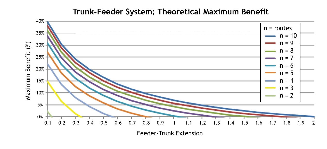
In this ideal case, there will be a generalized cost reduction from shifting from a direct service to a trunk-and-feeder service. This is shown in the next figure. The line below shows the slope ofi \( F_{pr}= { (N-1) ^2 \over (4*N_\text{route})} \)
For any combination above the line there is no benefit, and for any combination below the line there is a benefit to shifting to trunk-and-feeder under these conditions.
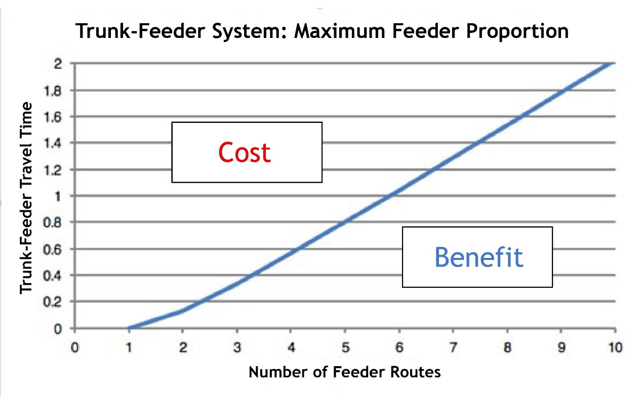
If all the possible outcomes are plotted as different combinations of the number of routes (\( N_\text{route} = n \) in the figure) and the feeder portion cycle time as a proportion of total cycle time \(F_pr\). It would be found that the benefits fall in the ranges shown in Figure 6.45.
The yellow line, for instance, indicates that the maximum benefit for a system where the direct service originally had only three routes (\( n = 3 \)), and the cycle time beyond the trunk is only 20 percent of the total cycle time (\(Fpr = 0.1\)).
The maximum total cost benefit is only 5 percent. In such circumstances, it will be nearly impossible to recover the other losses associated with trunk-and-feeder services from the benefits of optimizing the vehicle size.
This points to the fact that, if there are a lot of small direct service routes that overlap for a long distance with the trunk corridor, each route will have a relatively low demand and will optimally use small vehicles. If the small direct routes along the trunk route are turned into trunk-and-feeder services, customers on each low-demand route would share the use of a much larger vehicle, realizing returns to scale in the fixed cost of vehicles.
If the number of routes is low, the demand will be split among a smaller number of routes, so the original routes will already be using larger buses. Further, if the routes share only a short section of the trunk, the distance available for larger vehicles to reap benefits would be smaller, so there would be less benefit.
The smaller services with low demand have the greater benefits from joining the trunk-and-feeder system to achieve returns to scale. As with any collective, the more people who join, and the longer they remain members, the greater the benefit.
In summary, a corridor that has a long trunk and short feeder extensions and more routes, rather than fewer sharing the total demand, the greater the chances that a trunk-and-feeder system will bring benefits.
6.6.2.2Calculating the Benefits of a Trunk-and-Feeder System for Corridors with Multiple Routes of Different Characteristics
Usually, when planning a BRT system, most of the routes using a BRT corridor are different, and determining the benefits of a trunk-and-feeder operation in those conditions is complicated. This section outlines a methodology that will be applicable in some real-world conditions. In this scenario, to make things simpler, some of the same assumptions from the previous scenario still hold.
- A Trunk segment (and time) is the same for all routes.
- B No transfer time is required to get from the feeder vehicle to the trunk vehicle, just waiting time.
- C No extra time is required for vehicles to pull off the BRT trunk corridor and enter a transfer terminal.
- D PHtoCC = 0, there is no peak factor. In other words, it can be assumed that the demand is constant throughout the day, such that the effect of the peak factor index on the overall fleet size does not apply, so there is no fixed operating costs (Cf) disadvantage to converting to trunk-and-feeder services related to smaller fleet size.
However, in this case, each bus route is allowed to vary in the length that it overlaps the trunk corridor and in the cycle time.
In these conditions, one explores how to answer the following questions:
- Knowing that shifting all routes from direct services to a trunk-and-feeder system yields benefits, will there still be benefits if only some of the routes are changed to trunk-and-feeder?
- Is the maximum benefit obtained when all routes are converted to trunk-and-feeder, or when routes are selectively converted based on their demand profile?
- How is the optimum case determined?
We approach these questions in a similar manner to the subsection: Scenario II: Dwell Times and Demand Vary from Route-to-Route, and All Stations Are Similar, to decide which routes should be included in the busway, by calculating the benefits generated by shifting successive routes to trunk-and-feeder service starting from the condition where all routes are direct services. In order to analyze the theoretical behavior, the exercise allows for every possible bus size. In real operation planning, one has to select among the existing bus capacities (accepting design load factors up to 0.9 also comes into play) and calculate fixed costs and waiting costs (no longer equal) based on the resulting number of buses.
Each route has two basic characteristics that vary in this example:
- Maximum Load for route “i” \( = \text{MaxLoad}_i\);
- Cycle time on feeder part of route “i” \( = TC_{i\text{-feeder}} \)
With these two parameters, the following equations are obtained:
\( \text{MaxLoadperCycle}_{i\text{-direct}} =\text{MaxLoad} * TC_i\);
\[ \text{MaxLoadperCycle}_{i\text{-trunk}} =\text{MaxLoad} * TC_{i\text{-trunk}}\]
\[ \text{MaxLoadperCycle}_{i\text{-feeder}} =\text{MaxLoad} * TC_{i\text{-feeder}}\]
Where:
- \( \text{MaxLoad}_i \): Maximum hourly load for route “i” in the critical link;
- \( \text{MaxLoadperCycle}_{i\text{-direct}} \): Maximum load (or the number of passenger places required) on the direct service per cycle time for route “i”;
- \( \text{MaxLoad}_{i\text{-trunk}}\): Maximum load (or the number of passenger places required) on the trunk part of service per trunk cycle time (\(TC_{i\text{-trunk}}\)) for route “i”;
- \(\text{MaxLoadperCycle}_{i\text{-feeder}} \): Maximum load (or the number of passenger places required) on the trunk part of service per trunk cycle time (\( TC_{i\text{-feeder}}\)) for route “i”;
- \( TC_i\): cycle time for route “i,” could be also represented as TCi-direct;
- \( TC_{i\text{-feeder}}\): Cycle time in hours for a vehicle to complete one circuit of the feeder part of route “i”;
- \( TC_{i\text{-trunk}}\): Cycle time in hours for a vehicle to complete one circuit of the trunk part of route “i.”
This means that the feeder services should supply places during the peak hour to meet the maximum load on the critical link of the feeder route, which is assumed to be close to the terminal.
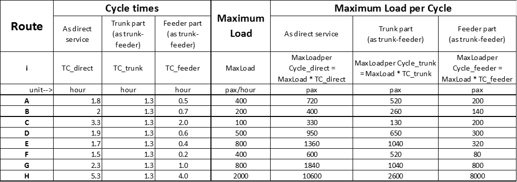
Our example considers eight routes as defined in Table 6.27 where the trunk part of all routes needs 1.3 hours and the assumption that \( TC_{i\text{-direct}} =TC_{i\text{-trunk}} + TC_{i\text{-feeder}} \) is still valid.
Table 6.27Example of Routes to Be Considered for Trunk-and-Feeder Service
Other variables that determine the optimal bus size and waiting costs are equal for all routes in the two alternatives (direct service and trunk-and-feeder service):
- BusFixedCost = US$30/per bus-hour;
- Renovation factor = 1.5;
- (Frequency) Irregularity = 0.3;
- Wait cost per passenger = US$12/hour;
- Design Load Factor = 0.85.
The equations are the same: Eq. 6.16a, Eq. 6.12, and Eq. 6.18 (taking into account the fixed operating costs per vehicle, \(\text{BusFixedCost}\)):
\[ \text{VSize}_\text{optimum}*\text{LoadFactor} = \sqrt{\text{BusFixedCost}*\text{MaxLoad}_\text{route} * TC \over {\text{Ren}_\text{route}*\text{Costwait} * 0.5 (1+Irr_\text{route})} } \]
\[ \text{WaitCost}_\text{route} = \text{Ren}_\text{route} * \text{Cost}_\text{wait} * 0.5 * (1+ Irr_\text{route}) *\text{LoadFactor} * \text{VSize} \]
\[ \text{FixedCost}_\text{route} = {\text{BusFixedCost} * \text{MaxLoadperCycle}_\text{route} \over { \text{VSize}_\text{route}*\text{LoadFactor}}} \]
Where:
- \( \text{VSize}_\text{optimum}\): Optimum vehicle size;
- \( \text{LoadFactor}\): Design load factor (usually 0.85).
- \( \text{BusFixedCost} \): Fixed operating costs per vehicle;
- \( \text{WaitCost}_\text{route} \): Total waiting time cost generated to the route users (in $);;
- \( \text{MaxLoad}_\text{route} \): Route demand on the critical link;
- \( \text{TC} \):Cycle time of the route;
- \( \text{Ren}_\text{route}\): Renovation factor of the route;
- \( \text{Costwait}_\text{route} \) Average user waiting cost ($/time);
- \( \text{Irr}\text{route}\): Irregularity index of the route; measure of the variance between the actual headways and the scheduled headways (usually near 0.3, see Section 6.3.9);
- \( \text{VSize}\): Vehicle capacity;
- \( \text{FixedCost}_\text{route} \): Total fixed operating cost for the route (in US$/hour) (\(=\text{WaitCostRoute}\) when \(\text{VSize}\) is optimum)
- \( \text{MaxLoadperCycle}_\text{route}\): Maximum demand across the critical segment of the route that will accumulate for the duration of one cycle during the busiest moment of the typical day (see Subsection 6.3.13);
In order to decide which should be changed, the routes should be situated in ascending order of places (\( \text{MaxLoadperCycle}_\text{feeder}\)) that each feeder route brings to the trunk service. Routes bringing fewer places to the trunk corridor will benefit more from being integrated into the trunk-and-feeder system, because these routes, in a direct service arrangement, will have the smallest vehicles.
Then the following should be calculated for each route:
- Optimal bus size and the sum of fixed plus waiting costs for operation as direct service;
- Optimal bus size and sum of fixed plus waiting costs for the feeder part of the route as if operated as trunk-and-feeder;
- Optimal bus size and sum of fixed plus waiting costs for the trunk assuming all routes classified as if operated as trunk-and-feeder.
With that, the overall benefits of fixed plus waiting costs of each alternative from splitting an additional route into separate feeder-and-trunk services can be calculated. The steps for the example are shown in Table 6.28.
Table 6.28Route Selection to Shift from Direct to Trunk-and-Feeder Service
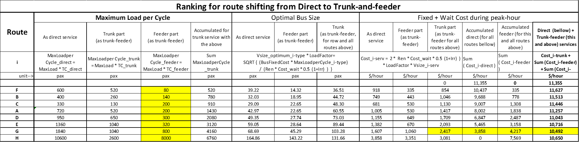
On the table, one can now compare scenarios. The first column “F” is a scenario where only the former direct service Route “F” has been converted to a trunk route and a feeder route. Then it is assumed that the remainder of the service is direct. The cost of servicing the remainder of the demand in the corridor with direct services is calculated thus:
- Total cost of waiting and fixed operating costs on the remaining direct service routes equals total cost of all direct service routes less the route converted to trunk-and-feeder, or:
\[ Cwf_\text{remaining direct lines} = Cwf_\text{all routes direct} - Cwf_\text{direct route F} \]
\[ = 11,355 – 918 = 10,437 \]
The total cost of a scenario where only Route F is converted to a trunk-and-feeder service, and all the remaining routes remain direct service routes, is just the cost of the trunk service, plus the cost of the feeder service, plus the cost of the remaining direct services, or:
\[ Cwf_\text{total Scenario F} = 854+335+10,437=11,627 \]
In the second scenario, row “B,” both Route F and Route B are converted to a trunk-and-feeder services, and all the other routes remain direct services. All of the columns are calculated in the same manner.
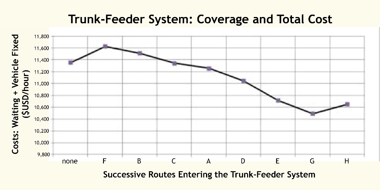
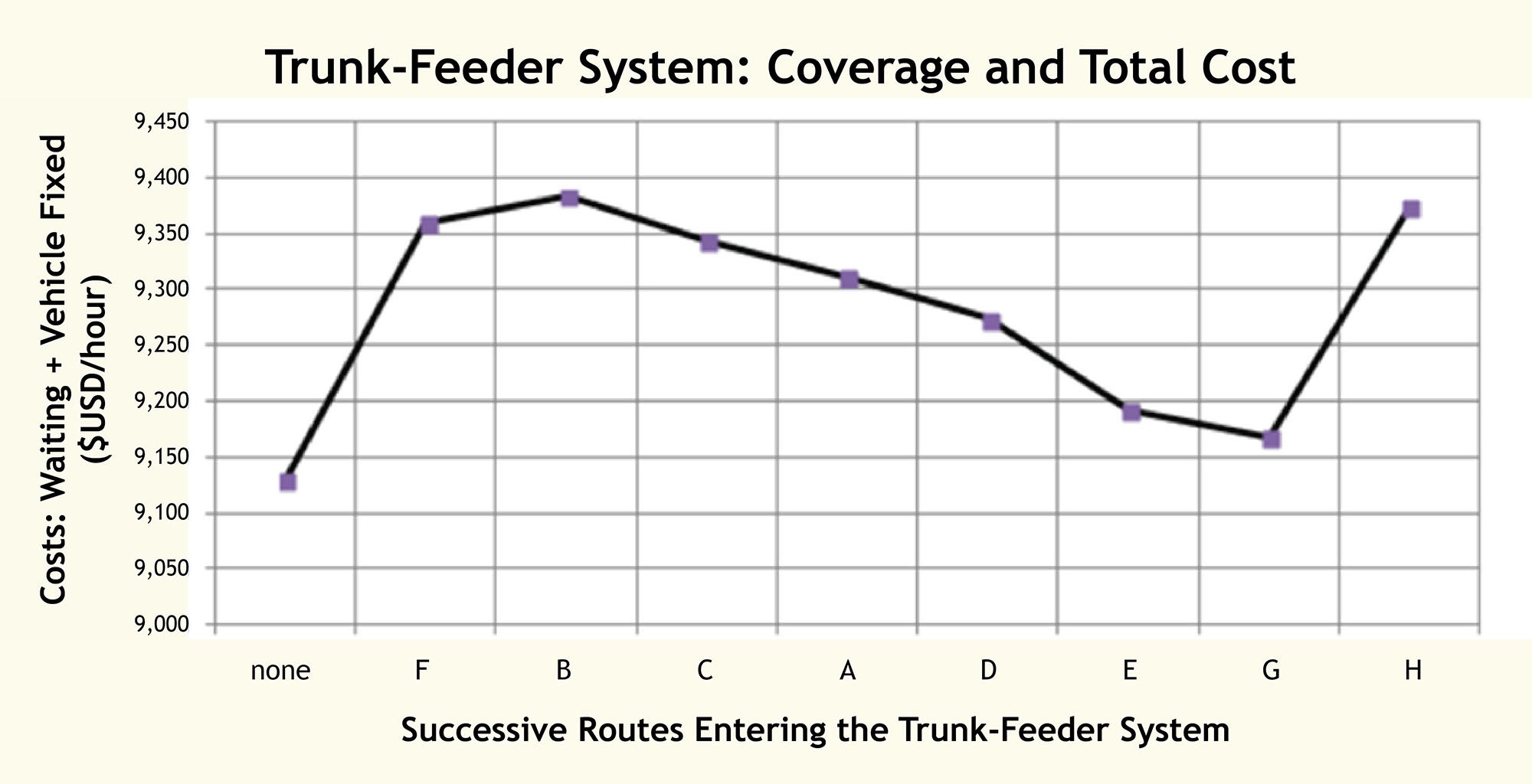
Unlike the costs of the feeder routes and the direct service routes, which will not change depending on how many routes there are, the trunk route will have decreasing costs the more routes that join the trunk-and-feeder service, as the maximum load and hence the vehicle size will increase the more small routes that join. The trunk-and-feeder system, under this specific set of assumptions, becomes more efficient than the direct-service-only system once the three best routes for conversion (F, B, and A) are added to the trunk-and-feeder service, as the total costs of the direct-service-only scenario (11,355) are greater than the trunk-and-feeder with F, B, and A scenario (11,342). The benefits continue to accrue as more routes are converted to trunk-and-feeder until Route H is added. Route H is particularly unsuited to trunk-and-feeder operations, because it has a very high demand on its own; has a very high frequency on its own; uses a very large vehicle size on its own; and continues well beyond the trunk corridor for some distance. With these characteristics, it is a prime candidate for a route that should continue to function as a direct service.
Figure 6.47 is a graph of the overall cost structure of each alternative:
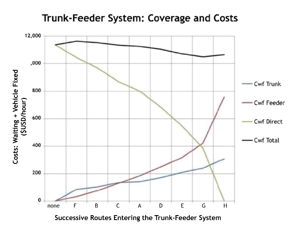
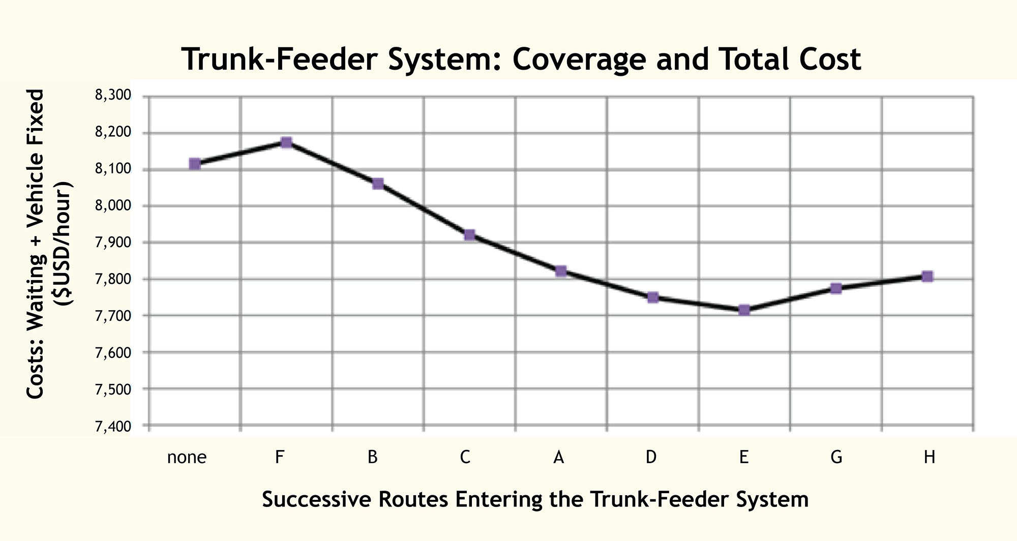
So as expected trunk-and-feeder system costs are growing, and normal route costs are decreasing. Figure 6.48 shows just the total cost:
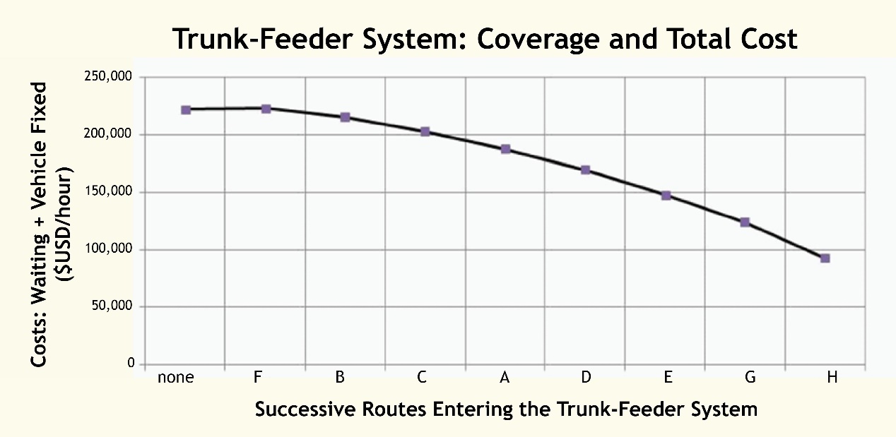
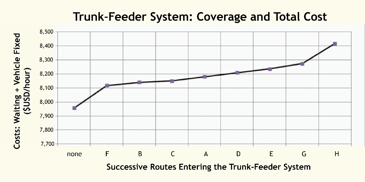
Box 6.4 Exercise to demonstrate the effectiveness of a trunk-and-feeder system
Continuing with the same methodology from above, one finds that if the trunk route is very long and carries a lot of demand, the costs will continue to fall as more routes are converted to trunk-and-feeder.
Conversely, if the trunk portion of the total route is very short, and most of the customers are going well beyond the trunk corridor, converting more routes to trunk-and-feeder will only increase overall system costs.
This exercise, while simplified from real-world conditions by a number of assumptions, demonstrates the general concept that the effectiveness of a trunk-and-feeder system depends on whether it makes sense for a critical mass of routes. Once it makes sense to convert a critical mass of routes to a trunk-and-feeder system, it becomes easier and easier to add more routes to the system profitably. Once trunk-and-feeder reaches critical mass, only very high volume routes continuing well beyond the trunk system are likely to still be profitably excluded from the trunk feeder system and retained as direct services. As such, there are mathematical reasons why there is a tendency toward systems with all direct services or all trunk-and-feeder services.
6.6.3Transfer and Terminal Delay
Splitting an existing direct service route into a trunk route and a feeder route will add several types of additional delay relating to the new required transfer. First, if transfer facilities are not located in an optimal location, or if access to the facility is poorly designed, vehicles will have to go out of their way to make the transfer possible, described as “negative distances,” increasing vehicle cycle times, and hence fleet requirements and operating costs. Second, transfers add significantly to customer travel times and discomfort since customers must walk from one bus route to the next. Avoiding transfer delays is often one of the main reasons discretionary riders elect not to use a system. Further, if transfers involve any form of physical hardship, such as stairs, tunnels, or exposure to rain, cold, or heat, then the system’s acceptability is even more compromised.
Not all transfers are equal. On one extreme are transfers located far from the trunk corridor involving slow and circuitous detours for both trunk routes and feeder routes to reach the transfer station, and lengthy walks across intersections and other obstacles unprotected from rain and sun. At the other extreme there are transfers made directly on a trunk corridor where many feeder services converge, with excellent terminal design involving minimal vehicle diversion and a simple few meters to walk across a comfortable, safe, and weather-protected platform. The quality of the transfer depends largely on the infrastructure and route design.
When considering whether to implement a trunk-and-feeder service, a direct service, or some combination, it is critical to calculate the likely delays caused by the forced transfer under the specific conditions being proposed for the system.
6.6.3.1Additional Passenger Delay Waiting for the Trunk Vehicle or Feeder Vehicle and Boarding and Alighting Again
When customers on a former direct service route now need to take a feeder vehicle and transfer at some point to a trunk vehicle, and this transfer point tends to be near where the bus route is at its maximum load, the maximum load of customers will now have to wait for the trunk vehicle in the morning and the feeder vehicle in the afternoon. These customers will face a waiting cost of half the headway of the trunk, or half the headway on their feeder route, depending on which direction they are going.
Since customers have to alight from the first vehicle and board a second one, there is an additional boarding and alighting delay per customer who needs to transfer. This additional delay will simply be the total boarding and alighting delay at the transfer station multiplied by the total number of transferring customers.
6.6.3.2Extended Vehicle Running Time Due to Route Modifications Required by the Suboptimal Location of the Transfer Terminal
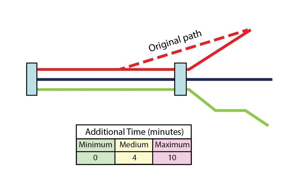
In all of the examples of trunk-and-feeder systems proposed in this section, all the routes pass a common point where they would diverge, so the location of a transfer terminal was simple and caused no additional travel time penalty. However, in most cases, the location of the terminal will serve some routes better than others. There will be some routes that will be pulled off their original route to reach a new common terminal point. In Figure 6.53, one of three vehicle routes is diverted from its original path because the terminal is not located where it originally departed the BRT corridor. This causes additional delay for all customers and additional operating time and cost for the vehicle operator. Some empirically observed ranges of additional minutes of running time on a route have been shown, but this will need to be measured on a route-by-route basis.
In addition, there is often no land readily available directly on the trunk corridor, so the terminal will need to be located where lower-cost land is available at some larger distance from the original trunk route. Terminals typically require a lot of land. In addition to accommodating other feeder services, terminals are places where vehicles turn around or park during off-peak periods (staging areas), and that requires space, too.
In most real-world cases, instead of placing a terminal at the natural convergence point of the existing bus routes, the terminal is located some blocks away on a piece of land owned by the municipality or that can be acquired otherwise at low cost. This adds two types of additional delay. It creates extra travel distance, possibly for both the trunk and the feeder vehicles, and it doubles the cycle time for vehicles traveling from the original corridor.
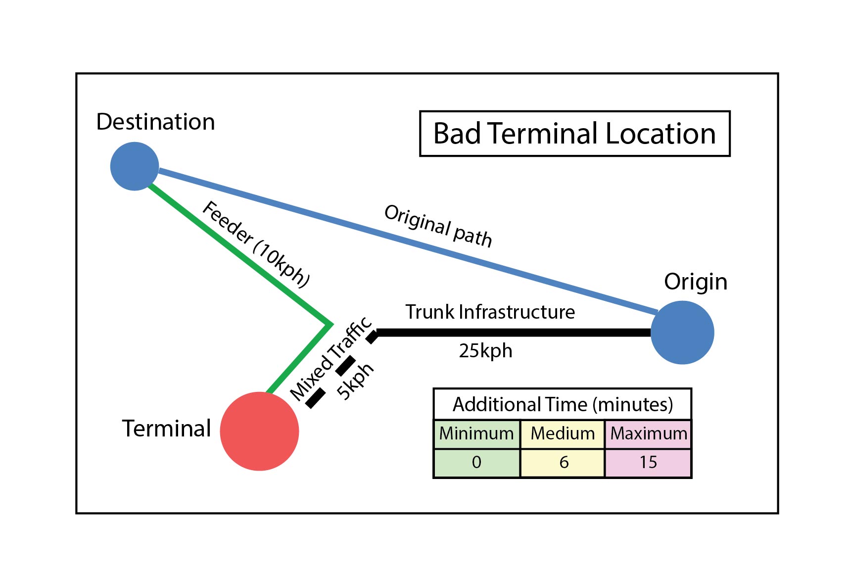
If the BRT trunk infrastructure is not extended all the way to the terminal, as is sometimes the case, the reduced speeds of the additional travel distance also need to be factored into the additional delay caused by the terminal being off corridor. Often, these access and egress roads around the terminal require complex new multiphase traffic signals, narrow, congested streets and other causes of slow speeds that did not affect the original direct service route that operated entirely on a major arterial.
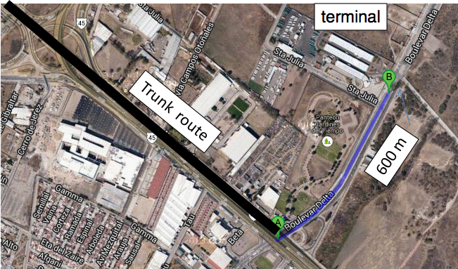
As an example of this situation, in León, Guanajuato, Mexico, the terminal is 600 meters away from the main trunk corridor on Lopez Mateos Avenue (Figure 6.55). In addition to the delay due to the 600-meter diversion, the speeds on the terminal access road are lower than on the original arterial, and additional signal delay was introduced in order to provide turning access to enter and exit the terminal.
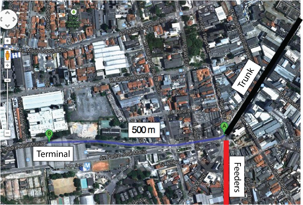
Another example is on Corridor 9 de Julho/Santo Amaro, in São Paulo, where the transfer terminal is 500 meters away from the natural connection point (Figure 6.56).
6.6.3.3Internal Circulation within the Transfer Terminal
The art of high-quality terminal design is not well known nor has it been systematized. In this planning guide, Chapters 25: Stations and 28: Multi-Modal Integration provide some very preliminary guidance, but optimizing a transfer terminal design is a critical area for further work.
Buses entering a transfer terminal often face significant delays caused by bus queues. Transfer terminals often include multiple platforms, as they are generally designed to accommodate multiple bus routes converging in one location. When poorly designed, there can be significant additional delays involved with vehicles entering the terminal and reaching their assigned platforms.
Transferring customers also face walks of varying distances and comfort depending on the quality of the terminal design. The best-designed trunk-and-feeder systems have feeder platforms immediately across from the trunk platforms, but not all terminals are so well designed. It is quite typical for a transfer terminal to require customers to needlessly climb up and down multiple stairways to reach their allotted boarding platform, when grade crossing would work just fine. If the terminal is large enough, it is of course impossible for all the feeder routes to be located immediately across the platform from a trunk platform, and the more feeder routes there are, the greater the likelihood that the customers will have to walk significant distances to reach their transfer route. Ideally, routes should be restructured and designed so that transfers can be made in several different stations, instead of concentrating all of them in just one location. Chapter 25: Stations and Chapter 28: Multi-Modal Integration also provide some preliminary guidelines for terminal design that can minimize this walking delay.
6.6.3.4Range of Likely Delays from Empirical Observations
Taking into account all six forms of transfer delay described in the previous four items, Table 6.29 provides some typical ranges for each variable.
Table 6.29Typical Ranges of Additional Terminal Delays
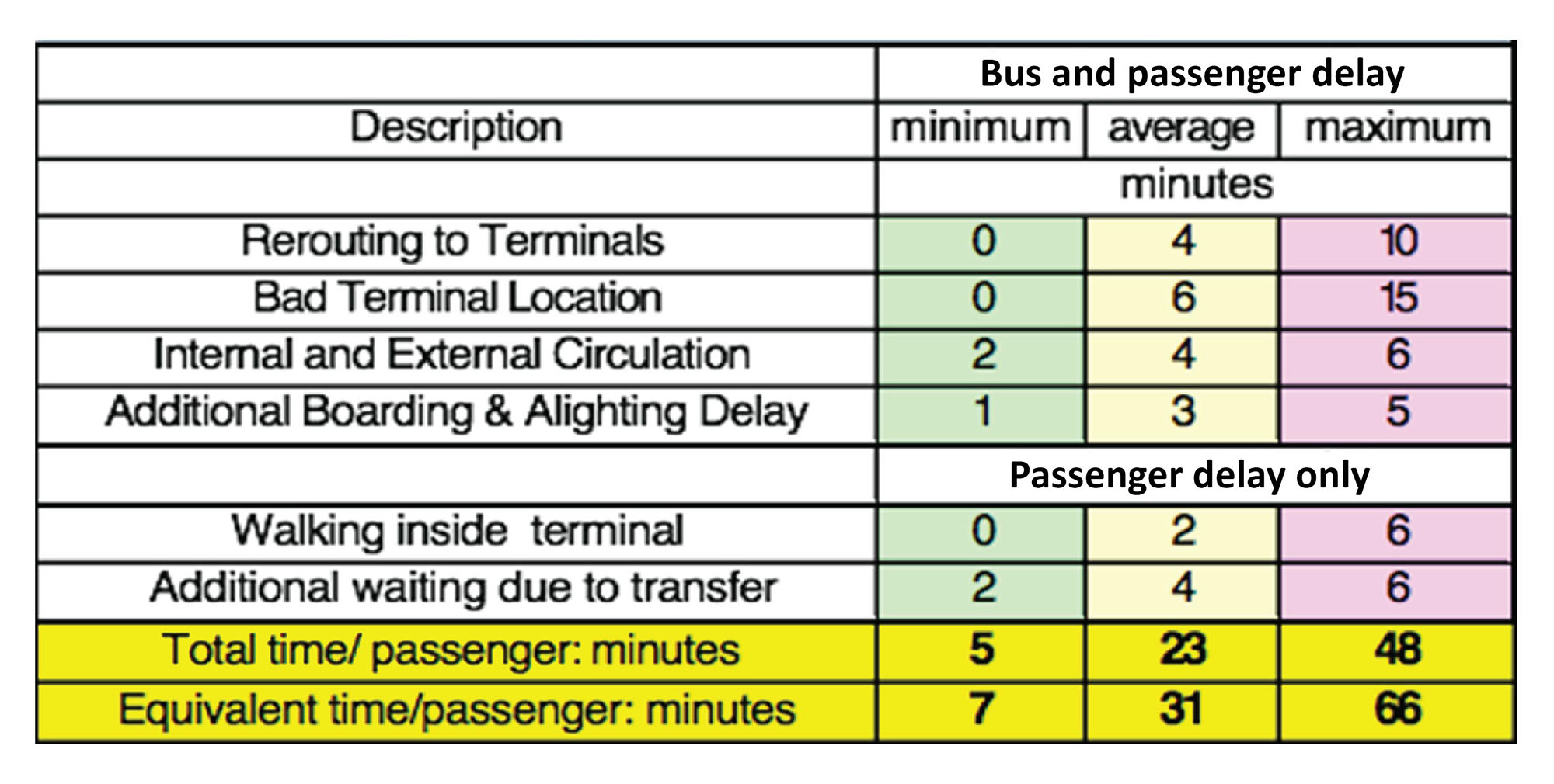
Some variables affect both the bus operating cost and the waiting time of customers, and other variables only affect customer waiting times. If a terminal is located directly on a trunk corridor and at a natural point of divergence for the feeder routes, there could be zero delay for customers and operators due to bad terminal location, but at worst both operators and customers could face very significant delays. Internal and external circulation time for the bus at the terminal virtually always adds some delay. Additional boarding and alighting time due to the transfer delays both customers and vehicles in all cases within predictable ranges.
The additional walking times inside the terminal will vary depending on the quality of the terminal design, and the additional waiting time due to the transfer will vary with the frequency of the trunk service and the feeder service within somewhat predictable ranges.
The total time in minutes per customer adds up with these causes of delay. The “equivalent time” per customer multiplies walking time by three, because people generally do not like to walk, and it multiplies waiting time by two, because people generally do not like to wait. In other words, following standard cost-benefit analysis practice, these two types of delay are weighted based on customers’ empirically observed willingness to pay to avoid these types of delay.
As a result of this transfer penalty, an average trunk-and-feeder system starts with a disadvantage of twenty-three minutes of customer travel time per route converted. These additional delays also translate into increased cycle time (\(TC\)), which directly translates into increased fleet needs and increased operating costs. When added to the extra fleet needed to compensate for the peak hour correction factor and extra fleet required at the terminal for scheduling adjustments in real-world conditions, it is typical for trunk feeder systems to require from 11 percent to 66 percent additional fleet. In most cases, these extra costs will total something in the range of 34 percent of an additional cost for the trunk-and-feeder service, while the benefits from the larger vehicle use are going to be generally in a similar range only when the trunk is very long relative to the feeder route, and there are many very small routes converging.
While the general benefits of many elements of BRT accrue primarily during the peak period, the time lost at terminals has an adverse impact on cycle times and customer travel times throughout the day. As a result, the benefits of a trunk-and-feeder BRT system exist mainly during peak hours. From a cost-benefit perspective, the terminal losses are rarely possible to recover from the benefits of being able to use larger vehicles on the trunk corridor.
In summary, an excellent terminal project, located directly on the BRT trunk corridor at a natural convergence point, is a necessary but insufficient precondition for achieving any benefit from the conversion from a direct service to a trunk-and-feeder service.
6.6.4Avoiding Station and Platform Saturation
There are two additional factors to consider when deciding on whether to convert a direct service route to a trunk-and-feeder route: station saturation and platform saturation.
6.6.4.1Avoiding Station Saturation
It may be the case that some existing bus routes using a planned BRT corridor operate with very small vehicles that are not compatible with BRT trunk infrastructure, usually because the roads they use are too narrow or in too deteriorated a condition for BRT vehicle operation. In this situation, including this route as a direct service on a BRT trunk corridor is likely to be ill advised. This is because providing a direct service for a minibus, for instance, is likely to more rapidly saturate the trunk corridor.
If the methodology is followed as suggested in subsection Scenario II: Dwell Times and Demand Vary from Route-to-Route, and All Stations Are Similar, where routes are included inside the BRT infrastructure based on a metric that gives priority to those bus routes where the customers using that route consume the least time at the bottleneck station, then it is likely that a route in which only minibuses can operate due to the operational conditions off the trunk route would be excluded because that type of bus would consume a lot of time at the bottleneck station.
In Section 6.5, it was assumed that such a route would operate in parallel to the BRT infrastructure in mixed traffic. However, such a solution has two disadvantages. The first is that the demand from the route is lost to the BRT system, and the second is that the mixed traffic lanes on the BRT corridor are more likely to face saturation. As such, in those conditions, it may be desirable to convert that direct service route into a trunk route and a feeder route.
The degree to which that specific route is likely to congest the bottleneck station can be calculated using the formulas provided in Chapter 7: Capacity and Speed on capacity and speed. The determination of whether the route should be simply cut, converted to a feeder, or allowed to continue to operate in the mixed traffic lanes will depend on the availability of land for a transfer location; the importance of the route to the level of demand on the trunk route; the level of congestion in the mixed traffic lanes; and the degree to which the trunk route can handle the additional demand without saturating the bottleneck station.
6.6.4.2Avoiding Station Platform Saturation
Another possible reason to convert a direct service route to a trunk-and-feeder service is if there is a risk that the trunk station platforms would become overcrowded with waiting customers, though in this case the less drastic and more practical option would be simply to reconfigure the routes.
Lower frequency, direct service buses can cause more customers to have to wait on station platforms than high-frequency trunk services. For low-demand systems this does not cause any significant problem. However, at high levels of demand, the station platform can become overcrowded and become saturated.
As such, there are limitations to the number of direct routes that can operate on the same trunk bus stop unless stations can be sized to handle the required volumes of waiting customers. While external fare collection, at-level boarding, multiple and large doors, and large vehicles have increased station capacity markedly (the subject of the next chapter), these features have not made any progress in reducing the space consumed by waiting customers.
In order to show the difference, begin by calculating the average number of passengers waiting for one route (\(Pwait_i\)) by:
Eq. 6.47
\[ P_{w i}= {P_{b i} \over F_i} * {(1+Irr_i) \over 2} \]
Where:
- \( P_{w i} \): Passengers waiting for route i at given station (passengers/hour);
- \( P_{b i} \): Boarding passengers in route i at given station (passengers/hour);
- \( F_i \): Frequency of route “i” (vehicles/hour);
- \( Irr_i \): Irregularity index of route i.
Then, the total number of passengers waiting at the station (Pwait) is given by:
Eq. 6.48
\[ P_{w total} = \sum_i {Pb_i \over F_i} * {(1+Irr_i) \over 2} \]
Where i is all the routes that use the station.
In other words, the number of customers that are likely to end up waiting on a platform will be the sum total of all of the boarding passengers per route per hour at that station divided by the frequency and then multiplied by the risk of irregular arrival of the bus.
For example:
\( P_{b i} \): 120 passengers/hour ;
\( F_i \): 6 vehicles/hour;
\( Irr_i \): 0.3 .
\[ P_{w i} = { {120 \over 6} * (1+0.3) \over 2} =13 \]
It might be expected that at any given time there would be 13 passengers accumulating for boarding in route i.
If there are 20 similar direct routes using the same sub-stop, there will be on average 13 passengers at that bus stop for each route at any given time.
So,:
\[ P_{w\ \text{direct}} = P_{w\ \text{total}} = 20 * 13 = 260 \]
There will be 260 passengers on the station platform at any given time.
To accommodate these passengers, normally one would want at least one square meter for every 2 passengers waiting. Also consider usable platform width minus 1 meter (0.5 m “buffer” on both sides), minus 1 meter for circulation space for up to 2,000 passengers per hour (1 meter of width is required per 2,000 circulating passengers per hour) to be the usable waiting space. Usually the length of the docking bay is considered the usable length.
Therefore, to accommodate just the waiting area for 260 passengers, and assuming circulating passengers are less than 2,000 per hour, one would need 260/2 = 130 square meters, or a platform 6 meters wide and 33 meters long, or 7 meters wide and 26 meters long, or 9 meters wide and 22 meters long, and so on.
If these 20 direct services routes (120 buses) were converted into just one trunk route with a frequency of 60 articulated buses per hour (cutting the frequency in half by doubling the size of the buses), the number of boarding passengers per hour into the one trunk route would be:
\[ P_{b i} = 120 * 20 = 2400 \]
And the average number of waiting passengers at each trunk station will be:
\[ P_{w\ \text{trunk}} = P_{w\ \text{total}} = { {2400 \over 60} * (1+0.3) \over 2} = 26 \text{passengers} \]
As people can take the first bus that comes along, fewer passengers accumulate on the platform waiting for their bus. In this scenario, trunk-and-feeder reduces the number of passengers waiting on each platform by 90 percent (from 260 to just 26) due to the frequency and size of the vehicles. Thus, the station platform only needs to be 13 meters long and 4 meters wide to comfortably accommodate the waiting passengers. Indeed, this is the more common situation, where the station length is determined not by the number of waiting passengers, but by consideration of the BRT station saturation from stopping buses, since the platform length required for 60 large buses per hour will be at least 40 meters. If there is limited space along the trunk route and sufficient space at the terminals, there will be some advantage to relocating these waiting passengers from a congested trunk platform to a transfer terminal.
When designing BRT stations, calculate the expected density of waiting customers based on the proposed service plan, and ensure that the length and width is adequate to serve both vehicle movements and waiting customer requirements. As the Guangzhou BRT is the highest capacity direct service BRT system in the world, it is worth looking at the station-sizing ramifications of its direct service in Figure 6.57.
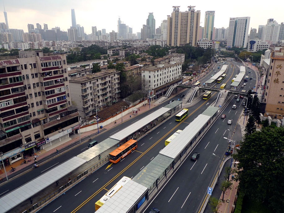
In Guangzhou, the design parameter was to provide for two passengers per square meter. Each docking bay has 5 meters of platform width, of which 2.5 is usable for a waiting area, and each waiting area per docking bay is 20 meters long. As such, each waiting area per bus is \( 20 \text{m} * 2.5 \text{m} = 50 {\text{m}}^2 \). With eight docking bays, the station can support up to 100 passengers per docking bay, and 800 passengers in total.
It was not easy, however, to convince the authorities to allocate 5 meters of road right-of-way to the station platform, although 5 meters is the average. A station narrower than 4 meters is not recommended for a bidirectional station. In very space-constrained locations, a small station with just 3 meters of width and 20 meters in length can only support around 60 passengers per hour.
6.6.5Conclusion: When to Consider Converting Direct Services to Trunk-and-Feeder Services
The large number of variables to consider when deciding whether to split existing direct services into trunk-and-feeder services makes it difficult to provide a single unified formula for making such a determination. Commercial public transport simulation software is not equipped to handle the sorts of multivariate analyses presented here either. The number of possible alternative service plan scenarios to test is so great that service planners need to follow some basic rules of thumb to create a set of scenarios for testing with a public transport demand model. As such, most of these decisions will need to continue to rely on good judgment assisted with the basic approaches and tools provided, aided by public transport software models only after many of the critical decisions have already been made.
The following provides a brief summary of these rules, based on the preceding discussions.
- Trunk-and-feeder systems require additional fleet due to the peaked nature of demand.
Trunk-and-feeder systems require larger fleets to accommodate the same number of customers. The more peaked the demand, the more additional fleet that the trunk- and-feeder service will require. In normal operating conditions, real-world observations indicate that the additional fleet required to convert a direct service into a trunk-and-feeder service will be in the range of 11 to 15 percent. If demand is heavily peaked, slightly more vehicles may be needed. If demand is less peaked, slightly fewer additional vehicles will be required.
- Trunk-and-feeder systems allow the use of larger buses with lower operating costs per customer on trunk routes, assuming high occupancy levels.
The main benefit of the trunk-and-feeder system is the ability to use larger buses with lower operating costs per customer along high-volume trunk corridors. By consolidating the demand from a number of lower demand direct service routes, a trunk BRT might be able to operate very large articulated or even bi-articulated buses along the trunk corridor, allowing for potential operating cost savings. This savings is likely to be in the 15 to 30 percent range if the trunk portion of the route is long relative to the feeder portion (say, the length of most of the feeder routes are considerably less than 50 percent of the length of the trunk corridor), and a large number of direct service routes (say, greater than five) originally shared the demand along the trunk corridor.
- Trunk-and-feeder systems impose additional costs related to the required additional transfers.
Trunk-and-feeder systems impose a lot of additional costs on BRT services related to the need for an additional transfer. These additional costs manifest themselves during the peak hour as well as throughout the day.
First, if it is not possible to locate the transfer terminal very near to the trunk corridor at a natural point of route divergence, the buses and their customers will need to go out of their way to get to the transfer terminal. This directly increases both customer travel time and cost and vehicle operating time and cost.
Circulation within and around the terminal also tends to cause delays. Poor circulation might involve problems with buses approaching and operating within the terminal, or it might involve the way customers move within the terminal. Poor terminal design is common in public transport system design, and the number of skilled terminal designers is limited.
This transfer terminal-related delay is likely to add between 11 and 66 percent to the fleet required in a trunk-and-feeder service plan. In addition, in a well-designed terminal, customers could face five-minute delays, and in a badly designed terminal, an additional 48 minutes per transferring customer has been observed.
Transfer terminals also tend to have large construction costs and may require land acquisition and resettlement. Once constructed, the transfer terminals need personnel to manage, operate, clean, and maintain them, adding to operating costs.
- Trunk-and-feeder systems can mitigate against station saturation and station platform saturation.
If some bus routes cannot easily use buses that are fully compatible with BRT trunk infrastructure (such as minibus routes operating on narrow, poorly maintained roads), incorporating them into the trunk corridor as direct service routes will increase the risk that the trunk corridor stations will become saturated. It may be better to turn such routes into feeder routes.
Direct services also require customers on the trunk corridor to wait longer for their bus than trunk services. This results in more customers accumulating inside the station waiting for their buses. Trunk-and-feeder services will reduce the number of accumulating customers waiting for their buses, because more customers can take more of the routes operating on the trunk. This problem is more likely to manifest itself in high-demand systems.
The conditions under which the conversion of direct services to trunk-and-feeder services will bring overall benefits are fairly limited. Until recently, trunk-and-feeder systems were proliferating in conditions inappropriate to their use, and direct service options were being neglected. This can probably be attributed to the similarity of trunk-and-feeder services to rail services, and the application of service plans developed in Gold Standard systems like Bogotá to cities with different conditions, where trunk-and-feeder operations may make less sense. In the future, with more full-featured direct service and hybrid (i.e., Direct + Trunk-and-Feeder) BRT systems coming into existence, such as the new system in Lanzhou, Yichang, and other cities, more real-world data will become available for comparison of the relative merits of the two basic service planning approaches.