6.4Optimizing Vehicle Size and Fleet Size
The approach to service planning laid out in this guide generally assumes that the system operators can and will adjust the number of vehicles they operate per route, and the size of the vehicles used on each route, to best serve the demand on each route.
This section covers some basic formulas needed to calculate the vehicle fleet and optimal vehicle size. These are two critical considerations when making service planning decisions, so they are covered first. The two decisions have to be made at the same time, since the larger the vehicle, the smaller the fleet. The process of optimizing vehicle size and fleet size is an iterative one.
Selecting an appropriate vehicle size requires balancing the operational cost savings of larger vehicles with the social costs of customers having to wait longer for the next vehicle. There are returns to scale with larger vehicles; the cost per customer served tends to fall with size. Drivers usually represent a disproportionate share of vehicle operating costs, and as the number of drivers is generally fixed and does not change with vehicle size, the cost of the driver relative to the total customers tends to fall the larger the vehicle.
On the other hand, larger vehicles also directly translate into lower frequency, and lower frequency means longer waiting times. Therefore, the costs of these two effects need to be measured in specific conditions when selecting an optimal vehicle size.
Given the goal of having the lowest possible costs using the design load factor, if the vehicle size has been decided (there are only a limited number of options), and the route has been decided and its demand estimated, then the fleet size can be easily calculated. The fleet size is calculated based on the number of vehicles needed to serve the maximum customer load on the highest demand section of the corridor during the peak time, as is explained in detail below.
6.4.1Vehicle Sizing, Basic Concepts
Vehicle types for BRT systems are not infinite, and for vehicles to operate inside a BRT corridor, there is rarely such low demand that a vehicle smaller than nine meters is ever likely to make sense. While new models are being launched in this market, manufacturers do not make an infinite number of vehicle sizes that are compatible with BRT infrastructure, so in general the range of vehicle options is limited to those listed in Table 6.6.
Table 6.6Range of BRT Vehicle Options
| Type | Vehicle Length (meters) | Capacity (customers) |
|---|---|---|
| Minibus | 9 | 60 |
| Bus | 12 | 90 |
| Articulated | 18 | 150 |
| Bi-Articulated | 25 | 220 |
In practice, the number of systems that use 9 meter or bi-articulated buses is quite limited. Most BRT systems use either 12-meter buses or 18-meter articulated buses. Bi-articulated buses are very expensive, generally double the cost of an articulated bus, and their primary use is in corridors with very high demand with very limited road space. They were first introduced in Curitiba by Volvo, and since then some are also in use in Mexico City on the Insurgentes Corridor, in TransMilenio in Bogotá, and in Istanbul. A few new BRT systems are planning to use 9-meter buses, but so far none are operational.
Note that the relationship between the vehicle length and the vehicle capacity is roughly the length (in meters) minus three (meters for the driver/engine/stairs, etc.) times 10 (or 10 customers per meter of operable bus length), or:
Eq. 6.10:
\[ \text{V}_\text{Size} = (V_\text{Length} – 3) * 10 \]
Where:
- \( \text{V}_\text{Size}\): Vehicle capacity in passengers (also written “pax”);
- \( \text{V}_\text{Length}\): Vehicle length in meters.
At the early stages of planning BRT services, one generally looks at the highest demand routes currently using the planned BRT corridor, and measures the maximum load on the critical link, i.e., the highest demand segment during the peak period.
The vehicle capacity (VSize) should be roughly equal to the maximum hourly load per route on the critical link (MaxLoad) divided by the frequency (Freq), or:
Eq. 6.11a:
\[ \text{V}_\text{Size} = { \text{MaxLoad} \over \text{Freq} * \text{LoadFactor}} \]
Where:
- \( \text{V}_\text{Size}\): Vehicle capacity;
- \( \text{MaxLoad}\): Maximum hourly load on the critical link;
- \( \text{Freq}\): Frequency;
- \( \text{LoadFactor}\): Design load factor (usually 0.85).
This becomes clear by seeing the impact that vehicle size has on frequency:
Eq. 6.11b:
\[ \text{Freq} = { \text{MaxLoad} \over \text{V}_\text{Size} * \text{LoadFactor}} \]
Or a third format as follows:
Eq. 6.11c:
\[ \text{Freq} * \text{V}_\text{Size} * \text{LoadFactor} = \text{MaxLoad} \]
As examples of capacity:
To serve 4,500 passengers (per hour per direction) on the critical link, a corridor may have:
- 50 buses (per hour) capable of carrying 90 passengers each; or
- 30 buses (per hour) capable of carrying 150 passengers each; or
- 18 buses (per hour) capable of carrying 250 passengers each.
To serve 900 passengers (per hour), a corridor may have:
- 10 buses (per hour) serving 90 passengers each;
- 6 buses (per hour) serving 150 passengers each.
6.4.2Vehicle Sizing, Initial Iteration
For reasons that will be explained in greater detail below, it is generally optimal to have a frequency set at about twenty-two vehicles per hour per route, as this tends to minimize the irregularity with which vehicle services operate while also minimizing waiting time. Once the frequency is above thirty or so, irregularity becomes a serious problem. At that point, it is generally advisable to introduce additional routes (i.e., limited stop routes, or routes serving other off-corridor destinations) rather than simply continuing to increase frequency or procuring larger and larger vehicles.
Since the BRT-compatible vehicle options are fairly limited, and generally the MaxLoad is known on existing bus routes from frequency and occupancy counts, it is sufficient as a starting point to use that maximum hourly load to determine vehicle size needed for each route. If the existing public transport routes’ maximum load is known, some estimate of what demand will be like in ten years needs to be made, as the vehicle is likely to last ten years. A reasonably secure methodology is to double existing ridership on the route, and divide by twenty-two vehicles per hour (an optimal frequency).
Vehicle size can be determined by taking a given maximum load and dividing it by an ideal frequency of twenty-two vehicles per hour (Eq. 6.11a applied to the route):
Eq. 6.11d:
\[ \text{VSize}_\text{route} = { \text{MaxLoad}_\text{route}\over \text{Freq}_\text{route}* \text{LoadFactor}_\text{route}} \]
Where:
- \( \text{VSize}_\text{route} \): Vehicle serving the route capacity;
- \( \text{MaxLoad}_\text{route} \): Route demand on the critical link;
- \( \text{Freq} \text{route} \): Frequency of the route (ideal frequency suggested of 22 vehicles per hour);
- \( \text{LoadFactor} \): Design load factor (usually 0.85).
Using that formula as a preliminary first pass, Table 6.7 shows that, with a maximum load greater than 3,500 existing customers per route, and a maximum 10-year estimated future load of 7,000, a frequency of 22 vehicles per hour, and a load factor of 0.85, the route should be separated into separate routes. If the maximum load on the critical link of a BRT route is currently between 1,500 and 3,000, bi-articulated buses can be used, but splitting the route should also be considered, as bi-articulated buses are expensive to purchase and maintain. For current loads between 1,000 and 1,500, articulated buses should be considered. Most BRT systems have more than one route per BRT corridor.
Table 6.7Bus Size by Varying MaxLoad per Route Using the Ideal Frequency of Twenty-Two Vehicles per Hour: First Iteration for Bus Sizing
| Existing Max Load | Future Max Load | Optimal Size | Proposal |
|---|---|---|---|
| 3500 | 7000 | 374 | Split the route |
| 3250 | 6500 | 348 | Split the route |
| 3000 | 6000 | 321 | Split the route |
| 2750 | 5500 | 294 | Split the route |
| 2500 | 5000 | 267 | Split the route |
| 2250 | 4500 | 241 | Split the route |
| 2000 | 4000 | 214 | Bi-articulated or split route |
| 1750 | 3500 | 187 | Bi-articulated or split route |
| 1500 | 3000 | 160 | Bi-articulated or split route |
| 1250 | 2500 | 134 | Articulated |
| 1000 | 2000 | 107 | Articulated |
| 750 | 1500 | 80 | 12 meter bus |
| 500 | 1000 | 53 | 9 meter bus |
| 250 | 500 | 27 | 9 meter bus |
This very initial estimate takes into consideration the need to minimize irregularity, but it does not consider the more critical element in bus size optimization, namely the relative costs of waiting (which will be higher for larger buses operating at lower frequencies) and the fixed cost of vehicle operation (which will be lower per customer for larger vehicles). Final vehicle size optimization will need to weigh these relative costs before finalizing the size.
This should only be a first iteration of vehicle size optimization. These preliminary vehicle-capacity figures can be used to calculate the necessary fleet, before returning to a more detailed methodology of calculating the optimal vehicle size.
6.4.3Detailed Vehicle Size Optimization
Further along in the planning process, when the design team already has a general idea of the sorts of services that will operate and their likely maximum loads at the critical link should have been developed, the following approach gives a more refined methodology for calculating the optimal vehicle size. This approach initially assumes there is no limitation to the size of vehicles available, that limitation will be considered in the application examples.
Put another way, vehicle capacity should be set where the cost of waiting faced by the users of that route (WaitCost) added to the fixed operating costs (FixedCost) of the route are minimized.
The total wait cost for a route (\(\text{WaitCost}_\text{route}\)) can be written as a function of bus capacity (VSize), by replacing Equation 6.11a:
\[ \text{V}_\text{Size} = { \text{MaxLoad} \over \text{Freq} * \text{LoadFactor}} \]
with Eq. 6.2
\[ \text{Freq} = {\text{MaxLoad} \over {V_\text{Size} * \text{LoadFactor}}} \]
Resulting in Eq. 6.12:
\[ \text{WaitCost}_\text{route} = { {\text{MaxLoad}_\text{route} *\text{Ren}_\text{route} *\text{Cost}_\text{wait} * 0.5 * ( 1+ Irr_\text{route} ) } \over ( { \text{MaxLoad}_\text{route} \over {\text{LoadFactor}*\text{VSize}} } ) } \]
\[ \text{WaitCost}_\text{route} = \text{Ren}_\text{route} * \text{Cost}_\text{wait} * 0.5 * (1+ Irr_\text{route}) *\text{LoadFactor} * \text{VSize} \]
Where:
- \(\text{WaitCostRoute}\): Total waiting time cost generated to the route users (in $);
- \(\text{MaxLoadroute}\): Route demand on the critical link;
- \(\text{Renroute}\): Renovation factor of the route;
- \( \text{Costwait}\) Average user waiting cost ($/time);
- \( \text{Irr}\text{route}\): Irregularity index of the route; measure of the variance between the actual headways and the scheduled headways (usually near 0.3, see Section 6.3.9);
- \(\text{Freq}_\text{route}\): Frequency of the route;
- \( \text{V}_\text{Size}\): Vehicle capacity;
- \( \text{MaxLoad}\): Maximum hourly load on the critical link;
- \( \text{LoadFactor}\): Design load factor (usually 0.85).
This shows that the cost to the customer rises as frequency falls. Hence, from the customer’s perspective, the larger the vehicle, the more time he or she has to spend waiting for it. On a high-demand corridor, there is usually high frequency, and the wait will be short, but there will be many more customers suffering the wait.
Assuming the other values are known (and they are estimated once a service plan is proposed), this can be expressed as:
Eq. 6.13
\[ \text{WaitCost}_\text{route} = A * VSize \]
Where:
- \(\text{WaitCostRoute}\): Total waiting time cost to the route users (in $);
- \(\text{V}_\text{Size}\): Vehicle capacity;
- \(A\): Known constant value
\[ A =\text{Ren}_\text{route} * \text{Cost}_\text{wait} * 0.5 * (1+ Irr_\text{route}) *\text{LoadFactor} \]
At the same time, fixed operating costs do not vary with vehicle size: the cost of the driver; the cost of the bus company’s overhead, the minimum cost of fueling any vehicle, and maintaining any vehicle no matter its size.
So the total fixed costs of a route operation are only a function of the route fleet (as proposed in Equation 6.9:
\[\text{RouteFixedCost} = \text{BusFixedCost} * \text{Fleet}_\text{route} \]
The route fleet (the number of vehicles needed to serve a route) is, in turn, dependent on the vehicle capacity (VSize) according to the following:
Eq. 6.14:
\[ \text{Fleet}_\text{route} = {\text{MaxLoadperCycle}_\text{route} \over {\text{VSize} * \text{LoadFactor}}} \]
Where:
- \( \text{Fleet}_\text{route}\): Number of vehicles needed to serve the route;
- \( \text{VSize}_\text{route}\): Vehicle serving the route capacity;
- \( \text{MaxLoadperCycle}\text{route}\): Maximum demand across the critical segment of the route that will accumulate for the duration of one cycle during the busiest moment of the typical day (see Subsection 6.3.13);
- \( \text{Freq}_\text{route}\): Frequency of the route (ideal frequency suggested of 22 vehicles per hour);
- \( \text{LoadFactor}\): Design load factor (usually 0.85).
In one extreme, if the route operated with a vehicle as large as the demand willing to cross the critical segment of the route that would be waiting for the duration of one cycle, only one vehicle would be needed.
As the vehicle operating on the route is smaller, the necessary fleet to carry all these customers will be larger, and so the fixed costs will be higher.
If we apply Equation 6.14 in Equation 6.11a we have:
\[ \text{FixedCost}_\text{route} = {\text{BusFixedCost} * \text{MaxLoadperCycle}_\text{route} \over { \text{VSize}*\text{LoadFactor}}} \]
Assuming the other values are known (and they are estimated once a service plan is proposed), this can be expressed as:
Eq. 6.15:
\[ \text{FixedCost}_\text{route} = {B \over \text{VSize} } \]
Where:
- \( \text{FixedCost}_\text{route}i \): Total fixed operating cost for the route (in $/hour);
- \( \text{VSize}_\text{route} \): Vehicle serving the route capacity;
- \( B \): Known constant value:
\[ B = {\text{BusFixedCost}*\text{MaxLoadperCycle}_\text{route} \over \text{LoadFactor}} \]
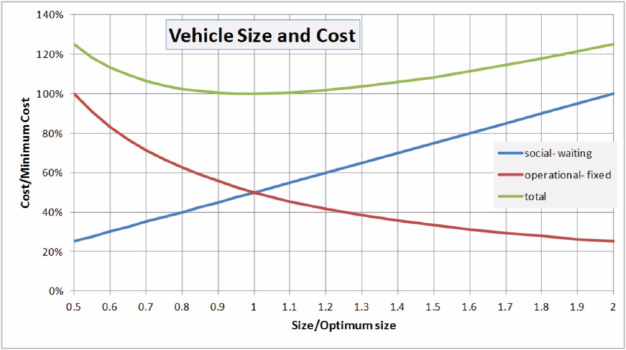
The graph in Figure 6.24 simply shows that the total social cost of waiting (the blue line) rises in direct linear proportion to the vehicle capacity, while the total fixed operational cost falls with vehicle capacity. The minimum total cost will be where Cw total (1 hour) = Cf total (1 hour).
The vehicle size that minimizes the cost of waiting imposed on the users (WaitCost) added to the fixed operating costs (FixedCost) to a given planned route is a vehicle size where FixedCost and WaitCost are equal.
\[ {{d(\text{WaitCost}_\text{route} + \text{FixedCost}_\text{route})} \over {d(\text{VSize})}} = { {d( A * \text{VSize} + {B \over \text{VSize}} )} \over {d(VSize)} } = A - {{B} \over {\text{VSize}^2}} =0 \]
\[ A - { {B} \over {\text{VSize}^2} } = 0 \Leftrightarrow A = {B \over { {\text VSize}^2}} \Leftrightarrow \text{VSize}^2 = {B \over A} \Leftrightarrow \text{VSize} = \sqrt{B \over A} \]
The vehicle capacity (VSize) that provides minimal added cost will result in:
\[ \text{WaitCost}_\text{route} = A*\text{VSize} = A * \sqrt{B \over A} = \sqrt{{A^2 *B} \over{A}} = \sqrt{A * B} \]
\[ \text{FixedCost}_\text{route} = {B \over \text{VSize}} = {B \over \sqrt{B \over A}} = {B \over \sqrt{B \over A}} ({\sqrt{B \over A} \over \sqrt{B \over A}})= \sqrt{B^2 \over {B \over A}} = \sqrt{A * B} \]
The optimal size is one where the waiting costs imposed on the last set of users from reducing the frequency is precisely equal to the benefits to the vehicle operator in terms of reduced operating costs of using a slightly larger vehicle. Any movement away from this point, and the total cost of customers waiting, plus operating costs, will be higher.
Therefore, optimal vehicle capacity (\( \text{VSize}_\text{optimum}\)) is:
\[ \text{VSize}_\text{optimum} = \sqrt{B \over A} = \sqrt{ {\text{BusFixedCost}*\text{MaxLoadperCycle}_\text{route} \over \text{LoadFactor}} \over {\text{Ren}_\text{route}*\text{Costi}_\text{wait}} * 0.5 * ( 1 + Irr_\text{route} * \text{LoadFactor}} \]
Eq. 6.16a:
\[ \text{VSize}_\text{optimum}*\text{LoadFactor} = \sqrt{\text{BusFixedCost}*\text{MaxLoadperCycle}_\text{route} \over {\text{Ren}_\text{route}*\text{Costwait} * 0.5 (1+Irr_\text{route}} } \]
Where:
- \( \text{VSize}_\text{optimum} \): Optimal size of vehicle to serve the route capacity;
- \( \text{BusFixedCost}\): Total fixed operating cost for the route (in $/hour);
- \( \text{MaxLoadperCycle}_\text{route}\): Maximum demand across the critical segment of the route that will accumulate for the duration of one cycle during the busiest moment of the typical day (see Subsection 6.3.13);
- \( \text{LoadFactor} \): Design load factor (usually 0.85);
- \(\text{Renroute}\): Renovation factor of the route;
- \( \text{Costwait}\) Average user waiting cost ($/time);
- \( \text{Irr}\text{route}\): Irregularity index of the route; measure of the variance between the actual headways and the scheduled headways (usually near 0.3, see Section 6.3.9);
6.4.4Vehicle Size Optimization Formula Applied
The following variables in Table 6.8 will be relatively constant, so the data can be collected either at the corridor level (Ren, Irr) or citywide (Costwait, BusFixedCost) and only needs to be done once. Below is some reasonable sample data, and because these tend to be consistent citywide, they can be turned into constants, except for the renovation rate, which needs to be calculated per corridor and is not consistent citywide.
Table 6.8Sample Data Used for Examples
| Variable | Symbol | Value | Unit |
|---|---|---|---|
| Fixed operating cost per bus | BusFixedCost | 30 | $/bus/hour |
| Waiting cost per passenger | Cost_Wait | 12 | $12/passenger/hour |
| Renovation factor on the corridor | Ren_route | 1.5 | |
| Irregularity Index on the corridor | Irr_route | 0.3 |
For this purpose, we can write Equation 6.16 as follows:
Eq. 6.16b:
\[ \text{VSize}_\text{optimum} * \text{LoadFactor}= \sqrt{\text{BusFixedCost} *\text{MaxLoadperCycle}_\text{route} \over \text{Ren}_\text{corridor} *\text{Costwait} * 0.5* (1+Irr_\text{city})} \]
\[ \text{VSize}_\text{optimum} * \text{LoadFactor}= \sqrt{ KA *\text{MaxLoadperCycle} } \]
Where:
- \(KA={\text{BusFixedCost} \over \text{Ren}_\text{corridor} *\text{Costwait} * 0.5* (1+Irr_\text{route})} \)
Using the data from the table and applying it to Equation 6.16, then:
\[ KA={30 \over 1.5*12*1+0.3*0.5 } = 2.56 \]
In other words, so long as the basic information about fixed costs, the renovation rate, the irregularity rate, the cost of waiting, and so forth are all calculated for the corridor, the difference in the vehicle size for each route will be a function of the difference in the maximum load over the course of a cycle time under each scenario, or put another way, the number of customer places (Pl) that the vehicles need to serve.
In applying this to Equation 6.16, then:
\[ \text{VSize}_\text{optimum} = \text{LoadFactor}=\text{MaxLoadperCycle}_\text{route} * 2.56 \]
In this way, the optimum vehicle capacity is simply a function of the demand over the course of the route’s cycle time that needs to be served under each scenario, times a constant, this of course must be divided by design load factor. Some examples of an application of this formula are shown in Table 6.9, where each row represents a different scenario.
For expediency in the examples below in Table 6.9, approximate values for MaxLoadperCycle are assumed rather than determining the actual value across multiple cycle times. A peak hour correction factor (PHtoCC) of 0.1 is also assumed, which is relatively typical. Other values are given in Table 6.9.
Using Equation 6.11 and the values in Table 6.9, optimal vehicle size (\(Cb_\text{optimum}\)) can be solved for, as shown in the last column of Table 6.9.
Eq. 6.17
\[ \text{MaxLoadperCycle} = \text{MaxLoad} * TC * [ 1 - \text{PHtoCC} * (\text{TC} -1) ] \]
Where:
- \( \text{MaxLoadperCycle}\): Maximum demand load per cycle time;
- \( \text{MaxLoad}\): Maximum hourly load on the critical link;
- \( \text{TC}\): Cycle time in hours.
- \( \text{PHtoCC}\): Nonnegative correction factor, the calibration of which is based on survey data, is discussed in Box 6.2.
Table 6.9Examples of Optimum Vehicle Size Derived from the Sample Data
| MaxLoad | TC | PHtoCC | MaxLoadperCycle | Size*LoadFactor |
|---|---|---|---|---|
| pass/h | hours | passengers | passengers | |
| 20 | 0.25 | 0.1 | 5 | 4 |
| 200 | 0.25 | 0.1 | 49 | 11 |
| 2,000 | 0.25 | 0.1 | 488 | 35 |
| 20 | 1 | 0.1 | 18 | 7 |
| 200 | 1 | 0.1 | 180 | 21 |
| 2,000 | 1 | 0.1 | 1,800 | 68 |
| 8,000 | 1 | 0.1 | 7,200 | 136 |
| 20 | 4 | 0.1 | 48 | 11 |
| 200 | 4 | 0.1 | 480 | 35 |
| 2,000 | 4 | 0.1 | 4,800 | 111 |
| 8,000 | 4 | 0.1 | 19,200 | 222 |
On this very wide range of maximum hourly loads and cycle times, optimum size assuming load factor equal to 1.0, varies from a car to a bi-articulated vehicle. If the optimal vehicle size (\(\text{VSize}_\text{optimum}\)) is four, in most cases the demand is too low to justify the procurement costs of special new BRT vehicles, and such small vehicles do not come in BRT-compatible forms, so are likely to congest the BRT corridor. Hence, this route would simply be excluded from the proposed BRT services, or turned into a feeder route for the BRT corridor. As BRT vehicle options are not actually infinite, once the optimal vehicle capacity is identified using the formula, VSizeoptimum will need to be set by rounding up to the nearest vehicle suitable for the BRT services and design load factor.
Table 6.10Examples for Determining Optimum Vehicle Size
| MaxLoad | TC | PHtoCC | MaxLoadperCycle | Size*LoadFactor |
|---|---|---|---|---|
| pass/h | hours | passengers | passengers | |
| 20 | 0.25 | 0.1 | 5 | Cut route |
| 200 | 0.25 | 0.1 | 49 | Cut route |
| 2,000 | 0.25 | 0.1 | 488 | 60 |
| 20 | 1 | 0.1 | 18 | Cut route |
| 200 | 1 | 0.1 | 180 | 60 |
| 2,000 | 1 | 0.1 | 1,800 | 90 |
| 8,000 | 1 | 0.1 | 7,200 | 150 |
| 20 | 4 | 0.1 | 48 | Cut route |
| 200 | 4 | 0.1 | 480 | 60 |
| 2,000 | 4 | 0.1 | 4,800 | 150 |
| 8,000 | 4 | 0.1 | 19,200 | 220 |
6.4.5Vehicle Fleet Optimization
One of the key purposes of developing a service plan is to know how many vehicles will need to be purchased. The factors involved in determining the operational size of the vehicle fleet include:
- Maximum hourly load on the critical link of a corridor (MaxLoad);
- Total cycle time (TC);
- Capacity of the vehicle (VSize);
- The degree to which demand is peaked (usually measured by a peak hour to cycle time correction factor, or PHtoCC as explained below);
- The need for a reserve fleet.
A reserve fleet needs to be added to the total fleet size, as vehicles will need to be serviced either preventatively or because they have broken down. As a rule, a reserve fleet is about 10 percent of the actual fleet needed to provide the service, although it can be lower than that.
6.4.5.1Vehicle Fleet Calculation with Uniform Demand
As a first estimate of the fleet needed to provide a new BRT service, the maximum load on the critical link of the existing bus routes currently using the BRT corridor during the peak hour should be calculated. The existing bus route lengths and cycle times also need to be calculated. This can usually be done at low cost with a GPS. From this information it is possible to estimate the current needed fleet.
Eq. 6.18
\[ \text{Fleet}_\text{route} = {{\text{MaxLoad}_\text{route} \cdot \text {TC}} \over \text{VSize} \cdot \text{LoadFactor}} \]
Where:
- \( \text{Fleet}_\text{route}\): Number of buses needed to serve the route;
- \( \text{VSize}_\text{route}\): Vehicle serving the route capacity;
- \( \text{MaxLoad}_\text{route}\):Maximum demand across the critical segment of the route that will accumulate for the duration of one hour, here is assumed constant;
- \( \text{TC}\): Cycle time in hours;
- \( \text{Freq}_\text{route}\):Frequency of the route;
- \( \text{LoadFactor} \): Design load factor (usually 0.85);
To provide an example, assume the following:
- \( \text{MaxLoad}_\text{route} = 224 \);
- \( TC= 2 \text{hours} \)
- \( \text{VSize} = 72 \);
- \(\text{Load Factor} = 0.85 \);
\[ Fleet = {224 * 2 \over 72 * 0.85} = 7.32 \]
If the formula produces a fraction, round up to the next integer, since vehicles have to be procured in units of one. So, in this scenario, the result is eight vehicles.
Once other service planning decisions have been made, and the route structure has been optimized and the vehicle size has been optimized, and future demand for this specific service scenario has been modelled, the fleet required for the new services should then again be calculated using this formula.
To explain this formula, begin with cycle time. If the total round-trip cycle time for the vehicle is two hours, at the end of one hour, the first vehicle will still have an hour to go before it can reach the beginning of the route and pick up a second load of customers. Since demand is uniform in this example, there will be the same number of customers on the critical link needing service in the second hour as during the first hour. As such, having a cycle time of two hours means that vehicles that travelled during the first hour will not be back to pick up customers on the critical link in the second hour. They will only just be starting their return trip. Thus, a second set of vehicles will be needed to serve the same demand on the critical link during the second hour while the first set of vehicles is returning. This is why one should multiply the MaxLoad by the cycle time. In this scenario, it is as if the number of customers is doubled.
If the cycle time were one, however, the same vehicle could return to the starting position after one hour to take the second hour of customers. Therefore, the same fleet can serve the demand on the critical link each hour (and in this scenario, the demand is the same each hour). Thus, cutting the cycle time to one cuts the needed fleet in half:
- \( \text{MaxLoad}_\text{route} = 224 \);
- \( TC= 1 \text{hour} \)
- \( \text{VSize} = 72 \);
- \(\text{Load Factor} = 0.85 \);
\[ Fleet = {224 * 1 \over 72 * 0.85} = 3.66 \]
As the fleet has to be rounded up to the nearest integer, it would be four vehicles.
For this reason deadheading, or running some buses in the contra-peak direction without customers, can reduce the total cycle time, and hence the fleet needed.
The size of the vehicle (VSize) is also important. Bigger vehicles can move the same number of customers with a smaller fleet. In the example above with a cycle time of two hours, if an articulated vehicle is used that can hold 180 customers, only three vehicles are needed:
- \( \text{MaxLoad}_\text{route} = 224 \);
- \( TC= 2 \text{hours} \)
- \( \text{VSize} = 180 \);
- \(\text{Load Factor} = 0.85 \);
\[ Fleet = {224 * 2 \over 180 * 0.85} = 2.923 \]
By increasing the vehicle size, the required fleet size decreases. This means fewer vehicles are required, but the result is that the frequency is lower, and customers will wait longer. Similarly, by decreasing the vehicle size, a larger fleet is needed, but frequency increases, and customers will not have to wait as long.
6.4.5.2Fleet Calculation with Peaked Demand
The above formula is good for rough calculations of fleet needs, but it is not sufficient to calculate the actual needed fleet in most real-world conditions where demand varies throughout the peak hours. Vehicles are expensive to purchase and operate, so more refined analysis is necessary.
To explain intuitively why the fleet needs for peaked demand are different than for uniform demand, the following example is useful. Assume a two-hour cycle time (TC) and sixty customers per vehicle (VSize), but this time, rather than assuming that MaxLoad is the same throughout three or four hours, from 6:00 a.m. to 9:00 a.m. assume that MaxLoad occurs only during the peak demand hour, let us say this is 6:45 a.m. to 7:45 a.m. just to get the idea.
With a two-hour cycle time, the first bus will return to pick up a second load of customers only after two hours. Thus, the total number of vehicles needed to serve the demand during the first peak hour is this plus the total needed to serve the demand during the second on-peak hour. A smaller fleet of vehicles is needed to serve that link during the second hour, because there are fewer customers.
The fleet needed is therefore not simply a function of the maximum load at the critical link and the vehicle size, but it is also a function of the cycle time and the degree to which demand is peaked.
Now, rather than simply calculating the fleet based on one single hourly demand, one must determine the maximum load on the critical link over the course of the cycle time, or MaxLoadperCycle. After the cycle time has passed, no more buses are needed as the first bus has returned to the beginning of the route.
The maximum load over the course of a cycle time is the total number of customers that will accumulate during one full route cycle time willing to cross the critical link on a given vehicle route. This can also be thought of as the number of passenger places that need to be served, or Pl.
Only so many vehicles are needed as would satisfy the customers that will accumulate before the first vehicle can complete its cycle and pick up a second round of customers. The original formula, Equation 6.5, can therefore be replaced with the following:
Eq. 6.19:
\[ \text{Fleet}_\text{route} = {\text{MaxLoadperCycle}_\text{route} \over \text{VSize}*\text{LoadFactor}} \]
Where:
- \( \text{Fleet}_\text{route}\): Number of buses needed to serve the route;
- \( \text{VSize}_\text{route}\): Vehicle serving the route capacity;
- \( \text{MaxLoadperCycle}_\text{route}\): Maximum demand across the critical segment of the route that will accumulate for the duration of one cycle during the busiest moment of the typical day (see Subsection 6.3.13);
- \( \text{Freq}_\text{route}\):Frequency of the route(ideal frequency suggested of 22 vehicles per hour);
- \( \text{LoadFactor} \): Design load factor (usually 0.85);
This then requires the development of a methodology for calculating the maximum load over the course of a specific cycle time.
At this point in the service planning effort, the service planner will have collected ridership data in fixed increments of time, such as fifteen-minute intervals, and determined the critical link. With that data, in order to calculate the fleet requirements, two questions must be answered:
- Given an expected cycle time (TC) period for a BRT route, what “TC period” of the day experiences the highest demand?
- How does one calculate fleet numbers based on the peak TC period?
In order to answer the first question, the example in Table 6.11 is a sample of fifteen-minute increment ridership data. In this example, the cycle time (TC) is one hour, so one should look for the peak hour.
Table 6.11Peak Period Critical Link Demand Profile for a Bus Route over Fifteen-Minute Increments and One-Hour TC Increments
| 15-Minute Time Increment | 15-Minute Observed Demand | One-Hour Time Increment | TC = One- Hour Accumulated Demand |
|---|---|---|---|
| 6:00–6:15 | 15 | N/A | N/A |
| 6:15–6:30 | 21 | N/A | N/A |
| 6:30–6:45 | 31 | N/A | N/A |
| 6:45–7:00 | 51 | 6:00–7:00 | 118 |
| 7:00–7:15 | 63 | 6:15–7:15 | 166 |
| 7:15–7:30 | 69 | 6:30–7:30 | 214 |
| 7:30–7:45 | 67 | 6:45–7:45 | 250 |
| 7:45–8:00 | 66 | 7:00–8:00 | 265 |
| 8:00–8:15 | 53 | 7:15–8:15 | 255 |
| 8:15–8:30 | 45 | 7:30–8:30 | 231 |
| 8:30–8:45 | 34 | 7:45–8:45 | 198 |
| 8:45–9:00 | 32 | 8:00–9:00 | 164 |
| 9:00–9:15 | 21 | 8:15–9:15 | 132 |
In Table 6.11, ridership data was collected and entered in fifteen-minute increments (“Fifteen-Minute Observed Demand”).
Here the column on the right shows the accumulated demand over each distinct one-hour (i.e., TC) period. For example, from 6:00 to 7:00, all of the demand observed passing the critical link from 6:00 to 6:15, 6:15 to 6:30, 6:30 to 6:45, and 6:45 to 7:00 has accumulated, for a total of 118. Since a full hour has not yet passed until 7:00, N/A is entered into the first three cells.
Now Question 1—what is the highest demand period for a given cycle time?—can be answered by looking at the table and choosing the hour with the greatest accumulated demand. In this case, it is 7:00–8:00 when accumulated demand reaches its maximum at 265 (the row highlighted in yellow). This is called the maximum load per cycle time (MaxLoadperCycle). If the cycle time is one hour, the final result is MaxLoadperCycle = 265.
If the cycle time TC were two hours, the table would look different:
Table 6.12Peak Period Critical Link Demand Profile over Fifteen-Minute Increments and Two-Hour TC Increments
| 15-Minute Time Increment | 15-Minute Observed Demand | Two-Hour Time Increment | TC = Two- Hour Accumulated Demand |
|---|---|---|---|
| 6:00–6:15 | 15 | N/A | N/A |
| 6:15–6:30 | 21 | N/A | N/A |
| 6:30–6:45 | 31 | N/A | N/A |
| 6:45–7:00 | 51 | N/A | N/A |
| 7:00–7:15 | 63 | N/A | N/A |
| 7:15–7:30 | 69 | N/A | N/A |
| 7:30–7:45 | 67 | N/A | N/A |
| 7:45–8:00 | 66 | 6:00–8:00 | 383 |
| 8:00–8:15 | 53 | 6:15–8:15 | 421 |
| 8:15–8:30 | 45 | 6:30–8:30 | 445 |
| 8:30–8:45 | 34 | 6:45–8:45 | 448 |
| 8:45–9:00 | 32 | 7:00–9:00 | 429 |
| 9:00–9:15 | 21 | 7:15–9:15 | 387 |
With a two-hour cycle time, the MaxLoadperCycle becomes 6:45–8:45 with a maximum demand of 448. Here, MaxLoadperCycle = 448.
If, on the other hand, the cycle time were fifteen minutes, the peak would be 7:15–7:30 and the MaxLoadperCycle = 69.
Now to address Question 2—how to calculate fleet numbers based on the peak TC period. There are two ways to obtain the fleet numbers. The simplest way is to determine the peak load over the course of the cycle time (\( L_\text{peak}[TC]\)), as shown above, and simply divide by vehicle capacity. That is:
Eq. 6.20:
\[ \text{Fleet}_\text{route} = {\text{MaxLoadperCycle}_\text{route} \over \text{VSize}*\text{LoadFactor}} \]
Where:
- \( \text{Fleet}_\text{route}\): Number of buses needed to serve the route;
- \( \text{VSize}_\text{route}\): Vehicle serving the route capacity;
- \( \text{MaxLoadperCycle}_\text{route}\): Maximum demand across the critical segment of the route that will accumulate for the duration of one cycle during the busiest moment of the typical day (see Subsection 6.3.13);
- \( \text{Freq}_\text{route}\):Frequency of the route(ideal frequency suggested of 22 vehicles per hour);
- \( \text{LoadFactor} \): Design load factor (usually 0.85);
So, for a TC of one hour, using the observed \(\text{MaxLoadperCycle}\) of 265, it is calculated that:
\[ \text{Fleet}(TC=1 \text{hour}) = { 265 \over 72 * 0.85} = 4.33 \]
Thus, the fleet needed for that peak cycle time is five.
So, for a TC of two hours, using the actual \(\text{MaxLoadperCycle}\) of two hours based on the data:
\[ \text{Fleet}(TC=2 \text{hours}) = { 448 \over 72 * 0.85} = 7.32 \]
This equates to a fleet of eight vehicles. A cycle time that is twice as long as another does not necessarily result in doubling the fleet. In this case, the cycle time increased from one to two hours, but the needed fleet went from five to eight, instead of to ten.
Box 6.2 How to determine correction factor from hour to cycle time (PHtoCC) based on load observations
When one is analyzing many existing or potential routes with different cycle times, it is cumbersome to calculate the necessary fleet in the more intuitive manner listed above. For this reason, this section offers another way to calculate the fleet with the use of a common peak to cycle factor derived from corridor specific data. The maximum-hour load only can be determined and then a Peak Hour to Cycle Correction Factor (PHtoCC) can be applied to that to expand the demand across the full array of possible cycle times. The calculation of the PHtoCC should be done per corridor and should be made separately for weekdays, Saturdays, and Sundays.
To calculate the peak hour to cycle correction factor, we present an example of a typical demand profile for the critical link on a BRT corridor during the morning peak derived from on Table 6.13.
Table 6.13Peak Period Critical Link Demand Profile
| Time | 15 Minute Loads | Cumulative |
|---|---|---|
| 6:00 a.m. | 15 | 15 |
| 6:15 a.m. | 21 | 36 |
| 6:30 a.m. | 31 | 67 |
| 6:45 a.m. | 51 | 118 |
| 7:00 a.m. | 63 | 181 |
| 7:15 a.m. | 69 | 250 |
| 7:30 a.m. | 67 | 317 |
| 7:45 a.m. | 66 | 383 |
| 8:00 a.m. | 53 | 436 |
| 8:15 a.m. | 45 | 481 |
| 8:30 a.m. | 34 | 515 |
| 8:45 a.m. | 32 | 547 |
| 9:00 a.m. | 21 | 568 |
| 9:00 a.m. | 21 | 589 |
| 9:15 a.m. | 19 | 608 |
| 9:30 a.m. | 35 | 643 |
| 9:45 a.m. | 24 | 667 |
| 10:00 a.m. | 29 | 696 |
| 10:15 a.m. | 25 | 721 |
| 10:30 a.m. | 25 | 746 |
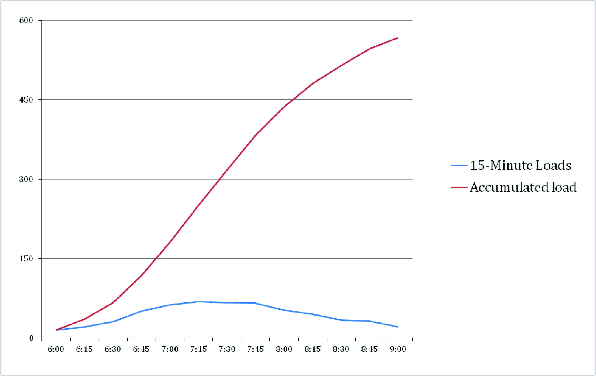
The blue line in Figure 6.25 is the number of customers every 15 minutes at the critical link, or the location where there is the maximum load (MaxLoad) of customers. The column labeled “15-minute loads” shows the number of people passing the critical link in 15-minute increments at different times. The red line is the accumulated load for the full peak period. The number of customers at 6:00 is fifteen. If the cycle time (TC) is two hours, the accumulation of customers at 8:00 (t + TC) is 436 minus the fifteen customers that were already on board at 6:00, or 421.
Note that the number of customers passing the critical link varies in each 15-minute interval. The maximum load for a 15-minute interval would be 69 at 7:15. This is equivalent to saying that the maximum load, or the number of customers that would be riding on vehicles past the critical link, if the cycle time were only 15 minutes, would be 69.
All of the possible time periods that are equivalent to the cycle time (TC) need to be tested to see which time period results in the maximum accumulated customers. To do this, create a table that simulates the number of customers that would accumulate per vehicle under different cycle times, such as in Table 6.14, where the first column to the right of the time cycle represents the observed loads at the critical link for every 15-minute interval. The second column places the 6:15 load next to the 6:00 load, and the 6:30 load next to the 6:15 load, and so on, because this is what the load would be for a 30-minute interval. It is not simply double the 6:00 a.m. demand, because the demand at 6:15 is different from the demand at 6:00 a.m. The third column places the 6:45 demand adjacent to the 6:30 demand, and so on.
Table 6.14Peak Period Loads by Cycle Time
| Time | 5 minute loads | Accumulated Passengers | Time | 15 minute loads | 15 min | 15 min | 15 min | 15 min | 15 min | 15 min | 15 min | 15 min | 15 min |
|---|---|---|---|---|---|---|---|---|---|---|---|---|---|
| 6:00 | 6 | 6 | 6:00 | 15 | 21 | 31 | 51 | 63 | 69 | 67 | 66 | 53 | 45 |
| 6:05 | 5 | 11 | 6:15 | 21 | 31 | 51 | 63 | 69 | 67 | 66 | 53 | 45 | 34 |
| 6:10 | 4 | 15 | 6:30 | 31 | 51 | 63 | 69 | 67 | 66 | 53 | 45 | 34 | 32 |
| 6:15 | 8 | 23 | 6:45 | 51 | 63 | 69 | 67 | 66 | 53 | 45 | 34 | 32 | 21 |
| 6:20 | 3 | 26 | 7:00 | 63 | 69 | 67 | 66 | 53 | 45 | 34 | 32 | 21 | 21 |
| 6:25 | 10 | 36 | 7:15 | 69 | 67 | 66 | 53 | 45 | 34 | 32 | 21 | 21 | 19 |
| 6:30 | 7 | 43 | 7:30 | 67 | 66 | 53 | 45 | 34 | 32 | 21 | 21 | 19 | 35 |
| 6:35 | 12 | 55 | 7:45 | 66 | 53 | 45 | 34 | 32 | 21 | 21 | 19 | 35 | 24 |
| 6:40 | 12 | 67 | 8:00 | 53 | 45 | 34 | 32 | 21 | 21 | 19 | 35 | 24 | 29 |
| 6:45 | 15 | 82 | 8:15 | 45 | 34 | 32 | 21 | 21 | 19 | 35 | 24 | 29 | 25 |
| 6:50 | 20 | 102 | 8:30 | 34 | 32 | 21 | 21 | 19 | 35 | 24 | 29 | 25 | 25 |
| 6:55 | 16 | 118 | 8:45 | 32 | 21 | 21 | 19 | 35 | 24 | 29 | 25 | 25 | 25 |
| 7:00 | 18 | 136 | 9:00 | 21 | 21 | 19 | 35 | 24 | 29 | 25 | 25 | 25 | 25 |
| 7:05 | 22 | 158 | 9:00 | 21 | 19 | 35 | 24 | 29 | 25 | 25 | 25 | 25 | 25 |
| 7:10 | 23 | 181 | 9:15 | 19 | 35 | 24 | 29 | 25 | 25 | 25 | 25 | 25 | 25 |
| 7:15 | 17 | 198 | 9:30 | 35 | 24 | 29 | 25 | 25 | 25 | 25 | 25 | 25 | 25 |
| 7:20 | 25 | 223 | 9:45 | 24 | 29 | 25 | 25 | 25 | 25 | 25 | 25 | 25 | 25 |
| 7:25 | 27 | 250 | 10:00 | 29 | 25 | 25 | 25 | 25 | 25 | 25 | 25 | 25 | 25 |
| 7:30 | 23 | 273 | 10:15 | 25 | 25 | 25 | 25 | 25 | 25 | 25 | 25 | 25 | 25 |
| 7:35 | 24 | 297 | 10:30 | 25 | 25 | 25 | 25 | 25 | 25 | 25 | 25 | 25 | 25 |
| 7:40 | 20 | 317 | 10:45 | 25 | 25 | 25 | 25 | 25 | 25 | 25 | 25 | 25 | 25 |
| 7:45 | 26 | 343 | 11:00 | 25 | 25 | 25 | 25 | 25 | 25 | 25 | 25 | 25 | 25 |
| 7:50 | 19 | 362 | 11:15 | 25 | 25 | 25 | 25 | 25 | 25 | 25 | 25 | 25 | 25 |
| 7:55 | 21 | 383 | 11:30 | 25 | 25 | 25 | 25 | 25 | 25 | 25 | 25 | 25 | 25 |
| 8:00 | 17 | 400 | 11:45 | 25 | 25 | 25 | 25 | 25 | 25 | 25 | 25 | 25 | 25 |
| 8:05 | 16 | 416 | 12:00 | 25 | 25 | 25 | 25 | 25 | 25 | 25 | 25 | 25 | 25 |
In Table 6.15, the 15-minute column is the same as the column above. The 30-minute column simply adds together the first two 15-minute columns from above, to give accumulated customers for a 30-minute interval. The 45-minute column totals the accumulated customers of the first three columns, and so on. In this simple way, a chart can be generated for the loads that would accumulate for each cycle time.
Table 6.15
Table 6.15Accumulated Passengers for Different Cycle Times
| Time | 15 min | 30 min | 45 min | 60 min | 75 min | 90 min | 105 min | 120 min | 135 min | 150 min | 165 min | 180 min |
|---|---|---|---|---|---|---|---|---|---|---|---|---|
| 6:00 | 15 | 36 | 67 | 118 | 181 | 250 | 317 | 383 | 436 | 481 | 515 | 547 |
| 6:15 | 21 | 52 | 103 | 166 | 235 | 302 | 368 | 421 | 466 | 500 | 532 | 553 |
| 6:30 | 31 | 82 | 145 | 214 | 281 | 347 | 400 | 445 | 479 | 511 | 532 | 553 |
| 6:45 | 51 | 114 | 183 | 250 | 316 | 369 | 414 | 448 | 480 | 501 | 522 | 541 |
| 7:00 | 63 | 132 | 199 | 265 | 318 | 363 | 397 | 429 | 450 | 471 | 490 | 525 |
| 7:15 | 69 | 136 | 202 | 255 | 300 | 334 | 366 | 387 | 408 | 427 | 462 | 486 |
| 7:30 | 67 | 133 | 186 | 231 | 265 | 297 | 318 | 339 | 358 | 393 | 417 | 446 |
| 7:45 | 66 | 119 | 164 | 198 | 230 | 251 | 272 | 291 | 326 | 350 | 379 | 404 |
| 8:00 | 53 | 98 | 132 | 164 | 185 | 206 | 225 | 260 | 284 | 313 | 338 | 363 |
| 8:15 | 45 | 79 | 111 | 132 | 153 | 172 | 207 | 231 | 260 | 285 | 310 | 335 |
| 8:30 | 34 | 66 | 87 | 108 | 127 | 162 | 186 | 215 | 240 | 265 | 290 | 315 |
| 8:45 | 32 | 53 | 74 | 93 | 128 | 152 | 181 | 206 | 231 | 256 | 281 | 306 |
| 9:00 | 21 | 42 | 61 | 96 | 120 | 149 | 174 | 199 | 224 | 249 | 274 | 299 |
| 9:00 | 21 | 40 | 75 | 99 | 128 | 153 | 178 | 203 | 228 | 253 | 278 | 303 |
| 9:15 | 19 | 54 | 78 | 107 | 132 | 157 | 182 | 207 | 232 | 257 | 282 | 307 |
| 9:30 | 35 | 59 | 88 | 113 | 138 | 163 | 188 | 213 | 238 | 263 | 288 | 313 |
| 9:45 | 24 | 53 | 78 | 103 | 128 | 153 | 178 | 203 | 228 | 253 | 278 | 303 |
| 10:00 | 29 | 54 | 79 | 104 | 129 | 154 | 179 | 204 | 229 | 254 | 279 | 304 |
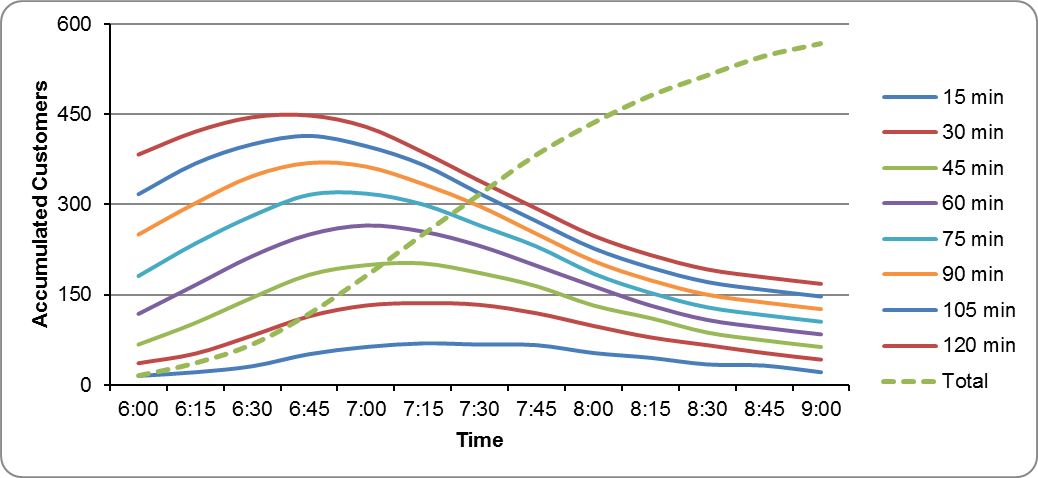
The maximum point on each curve shows the maximum accumulated customers, which is needed to derive the necessary fleet. Table 6.15 shows that the longer the cycle time, the more demand will accumulate before the same vehicle can get back to the beginning of the route to pick up more customers.
For the first example (the top brown-red line), different accumulated demands are graphed for different two-hour periods. Between 6:00 a.m. and 8:00 a.m. accumulated customers are 383 (the first data point at 6:00 a.m. on the top brown-red line). This is because at 8:00 a.m. there are already fifteen customers, and after two hours, 398 customers have accumulated, so enough vehicles to carry 383 (398-15) customers are needed. The accumulated customers from 6:00 to 8:00 are not the same, however, as the accumulated customers from 6:15 to 8:15, or from 6:30 to 8:30, etc. The top brown red line graphs the accumulated customers for each two-hour time increment are listed in Table 6.15 in the column labeled “120 minutes.” The peak period for this cycle time is about 6:45 to 8:45, when 448 passengers accumulate over two hours. Thus, for a two-hour cycle time, we can say that 448 is the MaxLoadperCycle = 448.
In each scenario, the load that needs to be accommodated with a fleet is the maximum load for each cycle time, or MaxLoadperCycle. In Table 6.15, the maximums are shown at the bottom of each cycle time. Because of the shape of the peak in demand, the maximum loads will vary depending on the cycle time. If the accumulated customers (load) per cycle time are divided by the cycle time, this gives the hourly load (MaxLoad [one hour]) for a specific cycle time.
Table 6.16Calculation of How the Maximum Load Varies with Cycle Time
| Hours | 0.25 | 0.5 | 0.75 | 1 | 1.25 | 1.5 | 1.75 | 2 | 2.25 | 2.5 | 2.75 | 3 |
|---|---|---|---|---|---|---|---|---|---|---|---|---|
| Cycle time (min) | 15 | 30 | 45 | 60 | 75 | 90 | 105 | 120 | 135 | 150 | 165 | 180 |
| MaxLoadperCycle | 69 | 136 | 202 | 265 | 318 | 369 | 414 | 448 | 480 | 511 | 532 | 553 |
| MaxLoad | 276 | 272 | 269 | 265 | 254 | 246 | 237 | 224 | 213 | 204 | 193 | 284 |
| ML | 1.04 | 1.03 | 1.02 | 1 | 0.96 | 0.93 | 0.89 | 0.85 | 0.81 | 0.77 | 0.73 | 0.7 |
If the maximum load for each cycle time is then further divided by the maximum load for a one-hour cycle time (265), then this gives an indicator (ML) that shows how much the maximum load for a specific cycle time varies from the maximum load for one hour. The peak hour to cycle correction factor (PHtoCC) is the slope of this line, indicating the degree to which the maximum load varies by the cycle time in general. In this way, a PHtoCC can be derived that can then be applied in the future to calculate the fleet needs for many routes of different cycle times.
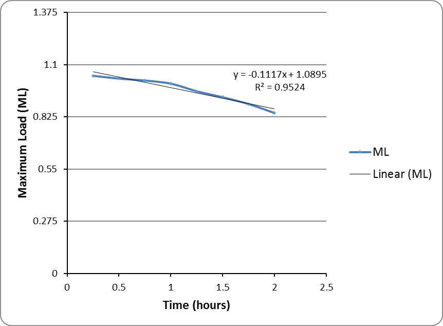
In Figure 6.27, rounding a bit, the PHtoCC = 0.11. MS-Excel will generate this number if instructed to provide the formula for a trend line when generating a graph.
Once the PHtoCC is known, the following formula may be used to determine MaxLoadperCycle for varying cycle times with peaked demand from the known MaxLoad, which is determined per hour. This formula is a simplification of a derivative, i.e., it describes a set of relationships that are linear in most real-world applications but that do not hold at the extremities, resulting in the previously presented.
Eq. 6.21a \( \text{MaxLoadperCycle} = \text{MaxLoad} * TC * [ 1 - \text{PHtoCC} * (\text{TC} -1) ] \)
Where:
\(\text{PHtoCC}\): Nonnegative correction factor, the calibration of which is based on survey data, is discussed in Box 6.2. The usual value is near 0.1;
- If \(\text{TC}\) is larger than one hour: correction \( 1 - \text{PHtoCC} * (\text{TC} -1) \) will result smaller than one;
- If \(\text{TC}\) is smaller than one hour: correction \( 1 - \text{PHtoCC} * (\text{TC} -1) \) will result larger than one;
- If \(\text{TC}\) is equal one hour: correction \( 1 - \text{PHtoCC} * (\text{TC} -1) \) will result in one;
- If \(\text{PHtoCC}\) is equal zero, there will be no correction.
And therefore the fleet needed for any route with any cycle time can be calculated as follows, by expanding Equation 6.14 with Equation 6.6b.
Eq. 6.21b
\[ \text{Fleet}_\text{route} = {\text{MaxLoadperCycle}_\text{route} \over {\text{VSize} * \text{LoadFactor}}} \]
\[ \text{Fleet}_\text{route} = {\text{MaxLoad} * TC * [ 1 - \text{PHtoCC} * (\text{TC} -1) ] \over {\text{VSize} * \text{LoadFactor}}} \]
Where:
- \( \text{Fleet}_\text{route}\): Number of buses needed to serve the route;
- \( \text{MaxLoad}\): Maximum hourly load;
- \( \text{VSize}_\text{route}\): Vehicle serving the route capacity;
- \( \text{Freq}_\text{route}\):Frequency of the route(ideal frequency suggested of 22 vehicles per hour);
- \( \text{LoadFactor} \): Design load factor (usually 0.85);
This approximation expands the peak one-hour load based on the degree to which the one-hour load is peaked within the full cycle time.
So, for a TC of two hours using the example from above, the maximum load is:
\[ MaxLoadperCycle=265*2*1-0.11*2-1=471.7\]
Hence, for a TC of two hours, the fleet needed is:
\[ 265*2*1-0.11*2-160 = 7.50 \]
\[ Fleet2hours=265*2*1-0.11*2-172*0.85=7.71 \]
The resulting 7.71 is a close approximation to the 7.32 used in the other formula, and again, one should round up to eight vehicles. (The discrepancy is because both formulas are simplifications to avoid the use of derivatives, to make the math easier in a way that is sufficient for most real-world uses.)
In most real-world cases, the peak hour to cycle correction factor (PHtoCC) is around 0.1. For a rough approximation, in a relatively normal peaked corridor, one can make a back-of-the-envelope adjustment by just using a generic peak factor such as 0.1, but it is better to calculate the actual peak factor. While this impact of the peak factor on the needed fleet is significant when calculating the fleet for any vehicle route, it makes a very big difference when a multitude of direct-service routes are severed into a trunk route and multiple feeder routes.