7.4Calculating Corridor Capacity
If I have the belief that I can do it, I shall surely acquire the capacity to do it even if I may not have it at the beginning.Mahatma Gandhi, political and spiritual leader, 1847–1948
7.4.1Corridor Capacity at Station Calculation
The provision of high capacities without creating undue saturation is a principal design consideration of most BRT systems. Once the bottleneck of the system is the station, the capacity of a BRT corridor is given by the capacity of its busiest station section, which is basically dependent on the vehicle size, load factor, and sum of service frequencies dwelling at each sub-stop with those who “jump” the station (direct services). Equation 7.20 below shows this.
Eq. 7.20 Corridor capacity at the station:
\[ \text{CorridorCapacity}_\text{at station} = \text{VSize} *\text{LoadFactor}*(\text{Freq}_\text{direct} + \sum_{i=1}^{N_\text{sub-stops} \text{Freq}_i}) \]
Where:
- \( \text{Corridor Capacity}_\text{at station} \): Number of people the corridor can transport through a given station section, in passengers per hour per direction (pphpd);
- \( \text{VSize} \): Maximum vehicle capacity;
- \( \text{LoadFactor} \): Average occupancy of the vehicles at the station, expressed as a proportion of the maximum vehicle capacity;
- \( \text{Freq}_\text{direct} \): Frequency of limited-stop services that skip the station under analysis;
- \( \text{Freq}_i \) Vehicle frequency at sub-stop i is the number of vehicles that dwells at all docking bays of sub-stop i during the evaluated interval (usually an hour);
- \( N_\text{sub-stops} \): Number of independent sub-stops in each station.
For a more generic evaluation, assuming the frequency in each sub-stop is the same, the corridor capacity at the station is:
Eq. 7.21 Basic formula for corridor capacity at station
\[ \text{CorridorCapacity}_\text{at station} = \text{VSize} * \text{LoadFactor} * (\text{Freq}_\text{direct} + \text{NSubstops} *\text{Freq}_\text{sub-stop}) \]
Table 7.2 shows sample corridor capacities for a range of common scenarios without limited-stop services. By varying only the vehicle capacity and the number of sub-stops per station, it shows just how powerful these two factors are in determining system capacity. It must be noted that the actual potential capacities for a given city will not be influenced by other system characteristics. But it should also be noticed that the table and the equation do not reveal anything about system speed.
Table 7.2BRT Corridor Capacity at Station Scenarios
| Vehicle capacity (passengers) | Load factor | Vehicle frequency per hour per sub-stop | Number of sub-stops per station | Capacity flow (passengers per hour per direction) |
|---|---|---|---|---|
| 70 | 0.85 | 60 | 1 | 3,570 |
| 160 | 0.85 | 60 | 1 | 8,160 |
| 270 | 0.85 | 60 | 1 | 13,770 |
| 70 | 0.85 | 60 | 2 | 7,140 |
| 160 | 0.85 | 60 | 2 | 16,320 |
| 270 | 0.85 | 60 | 2 | 27,540 |
| 70 | 0.85 | 60 | 4 | 14,280 |
| 160 | 0.85 | 60 | 4 | 32,640 |
| 270 | 0.85 | 60 | 4 | 55,080 |
| 160 | 0.85 | 60 | 5 | 40,800 |
| 270 | 0.85 | 60 | 5 | 68,850 |
Source: Institute of Transportation Studies, University of California, Berkeley
The value of sixty vehicles per hour at a sub-stop with one docking bay is a common and relatively easy way to achieve value—that is, one vehicle per minute. A regular bus stop (let us say a curbside stop in a congested mixed traffic environment) with space for two 12-meter vehicles loading simultaneously would handle 60 vehicles per hour, while the average number of boardings per bus is not bigger than 30 customers (which is one-third of such bus maximum capacity); we assume 20 seconds of dead time (dead time is shorter under congested conditions) and 3 seconds per boarding customer (which is achievable with one step boarding at one door as long as fare collection is in the middle the bus).
The tricky part of the design is achieving that frequency without forming queues at the station. For the example of the last paragraph, at a one docking bay capacity, one should expect a queue of 12 vehicles after one hour of operation, 24 vehicles after two hours of operation, and so on. If instead of an average of 30 customers boarding per bus, the average would be 20 customers boarding per bus, a saturation level of 75 percent, after one hour of operation the expected queue would be of 2.5 buses and of similar size after that. This still would mean an extra delay of two minutes for all customers inside the bus at this bus stop. The total time at the station would be three minutes instead of two. That is quite a lot if compared with TransMilenio (see the example illustrating Equation 7.1) where the time at a station for twenty customers to board would be twenty-one seconds.
The number of docking bays can also create serious problems, unless operating in a controlled convoy, a station split in two curbside stops as in the previous example (operating at a 75 percent saturation level) would have to be apart from each other by 100 meters to create queueing places for the buses (even the average queue is of 2 to 3 vehicles, it will likely reach 7 vehicles queueing behind the 2 already loading in the course of an hour of operation), otherwise the vehicles forming the queue for boarding at the front pole will block the exit of buses loading at the back pole, creating more queues, resulting in congestion.
7.4.2Detailed Capacity Calculation
While Chapter 6: Service Planning provided guidance on how to select routes to include on the corridor (Section 6.5.3) and to skip stations (Section 6.6.4) so that operational capacity was not surpassed, the following sections of this chapter (Sections 7.5 and 7.6) evaluate how system characteristics will affect operational capacity, so proper features can be selected to reach the required operational capacity.
The capacity calculation for a station given earlier (Equation 7.20), applied to the segment with the higher number of services, would give the system capacity.
If a design is proposed where saturations are above 40 percent, it can be considered above operational capacity and adjustments have to be made. As an example, let us consider a corridor where the demand study indicated that the boarding and alighting requirements per station in one direction at the morning peak hour are as given in Table 7.3, for the first and tenth years of operation.
Table 7.3Corridor Demand Example
| MORNING PEAK HOUR - YEAR 0 | MORNING PEAK HOUR - YEAR 10 | |||
|---|---|---|---|---|
| station | Boarding passengers (pax/hour) | Alighting passengers (pax/hour) | Boarding passengers (pax/hour) | Alighting passengers (pax/hour) |
| A | 824 | 0 | 1030 | 0 |
| B | 734 | 8 | 918 | 10 |
| C | 646 | 15 | 808 | 19 |
| D | 554 | 43 | 693 | 54 |
| E | 768 | 82 | 960 | 102 |
| F | 364 | 176 | 455 | 220 |
| G | 272 | 235 | 340 | 294 |
| H | 180 | 424 | 225 | 530 |
| I | 161 | 358 | 201 | 448 |
| J | 144 | 330 | 180 | 413 |
| K | 130 | 298 | 162 | 372 |
| L | 118 | 260 | 147 | 325 |
| M | 94 | 544 | 117 | 680 |
| N | 70 | 568 | 87 | 710 |
| O | 64 | 533 | 80 | 666 |
| P | 48 | 499 | 60 | 624 |
| Q | 43 | 199 | 54 | 249 |
| R | 34 | 214 | 42 | 267 |
| S | 19 | 230 | 24 | 288 |
| T | 0 | 250 | 0 | 312 |
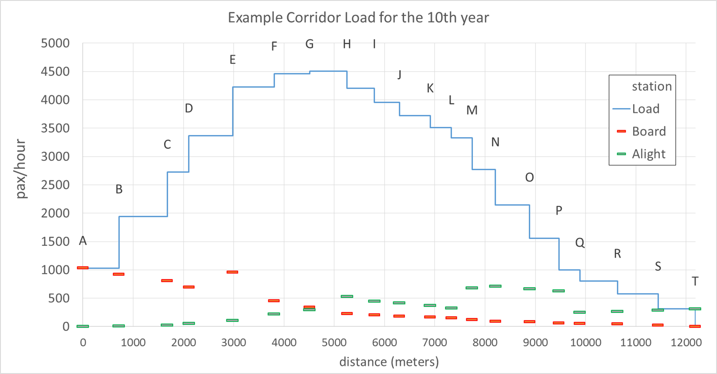
The load of all segments is already defined, as the load of the preceding segment plus boarding of preceding station minus alighting at the preceding station.
For the beginning year of operations (year 0), an initial service plan proposed a closed trunk corridor with twenty stations, with one service stopping at all stations. The service will be operated using a seventy-passenger vehicle with a headway of one minute.
The proposed standard station will have an elevated platform with external fare collection, resulting in boarding or alighting times of one second per customer (for either of the two vehicle doors).
The supply is defined as 4,200 pphpd (60 vehicles per hour multiplied by 70 passengers per vehicle) for the entire corridor. The system capacity, by using a design load factor of 0.85 in order to avoid overcrowding due to irregularity, is 3,570 pphpd.
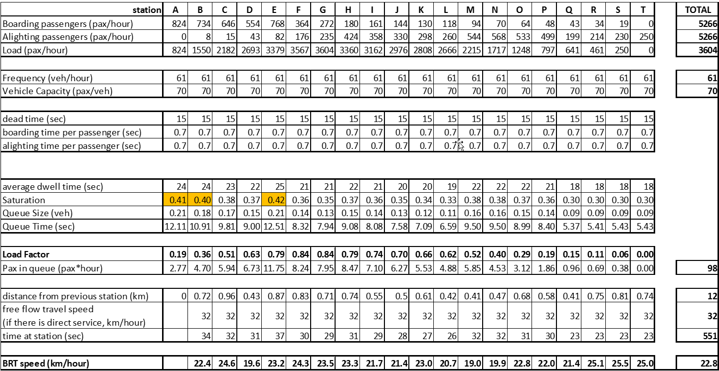
Table 7.4, which can be reproduced with the formulas discussed in the previous sections of this chapter, shows that the proposed solution leads to a load factor of 0.86 at the critical link, as well as saturation levels above the accepted limit.
Table 7.4Station Saturation at Example Corridor for First Year Initial Proposal
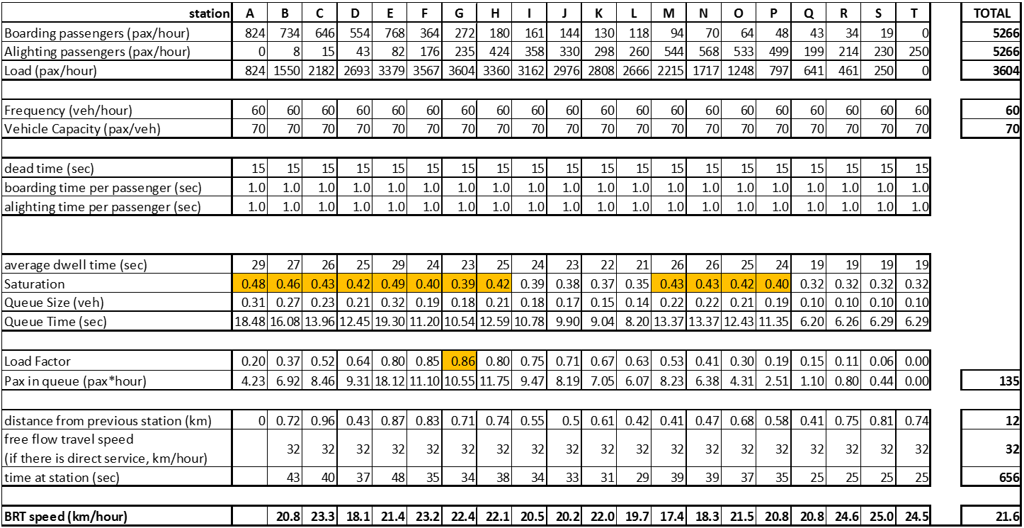
To reduce the load factor to the proposed value of 0.85, it is enough to raise service frequency to 61 vehicles per hour. While only one more bus per hour, this is nearly a 2 percent capacity increase.
If instead of using a 2-door vehicle, a 3-door vehicle is proposed, with a reduction of boarding or alighting time from 1.0 second per customer to 0.7 seconds per customer, then saturation gets closer to an acceptable level, as shown in Table 7.5.
Table 7.5Station Saturation at Example Corridor for First Year Second Proposal
If such levels were found at the tenth year of operation, one could tolerate this proposal, but as the demand will grow, this saturation is clearly not acceptable.
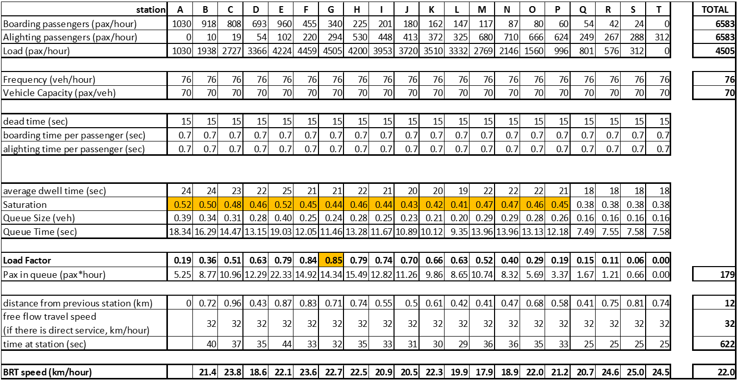
Indeed, looking at the MaxLoad for the tenth year of operation, 4,505 passengers per hour, after station G (shown in Table 7.6), one can tell that 76 vehicles per hour will be required (capacity equal to 4,522 pphpd), and with such frequencies, all stations will be at risk of experiencing severe congestion. The resulting times and speeds in Table 7.6 seem acceptable, but due to planning uncertainties, saturations above the 0.4 limit expose the system to breakdown.
Table 7.6Station Saturation at Example Corridor for Tenth Year First Proposal
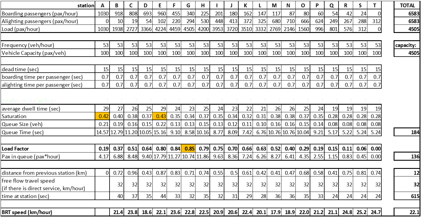
Vehicle sizes were determined for minimizing the sum of waiting and operating costs. By increasing vehicle size to increase operational capacity, waiting times would also increase, especially in the first years of operation. One of the objectives of the system is to reduce travel times door-to-door, so this has to be weighed in that light. Increasing the vehicle size to a 15-meter vehicle for 100 passengers, however, would allow some stations in the example to perform above operational capacity (4,505 passengers per hour with 53 vehicles per hour) in the tenth year of operation, as shown in Table 7.7, with a more acceptable saturation level.
Table 7.7Station Saturation at Example Corridor for Tenth Year Increasing Vehicle Size to 100 Passengers
Using an articulated 160-passenger vehicle would bring saturation at the critical station to a comfortable saturation level of 0.34. If the design included a fourth door, reducing boarding time to 0.5 seconds per customer, than saturation at the critical station would be 0.29. But in the first year, frequency would be twenty-six vehicles per hour (over a two-minute headway) and average wait time would be over one minute in the peak, and during the off-peak time this value would likely double or triple.
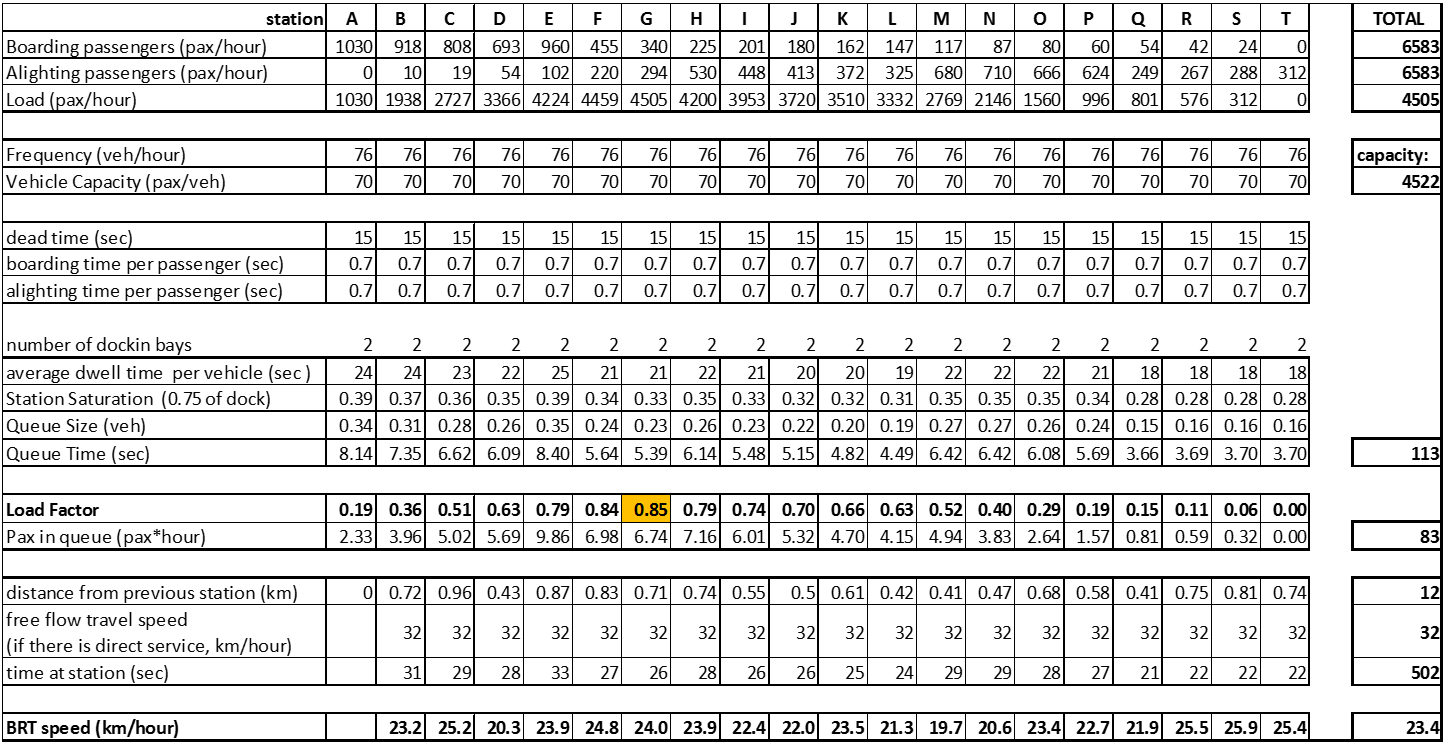
Without having to add overtaking lanes at the stations (although overtaking lanes may be feasible without affecting mixed traffic capacity if stations are properly located; see Chapter 24: Intersections and Signal Control), the only solution left keeping those vehicle sizes would be to use two docking bays per station, as shown in Table 7.8. As this is not a congested situation, dead times will not be heavily affected. What is expected is that a certain number of times (proportional to the queue size of Table 7.6), boarding will occur through the second platform of the station. Total passenger queueing time is significantly reduced from 136 hours to 83.
Table 7.8Station Saturation at Example Corridor for Tenth Year with Two Docking Bays per Station
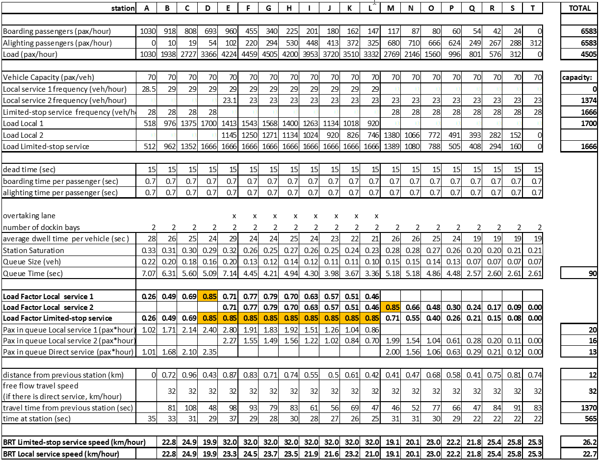
To consider the provision of overtaking lanes, one must look at the internal origin-destination matrix of the BRT system (in Table 7.9) to identify potential route splits to create limited services. Ideally, these limited routes should have a headway between 2.5 to 3 minutes in order to reduce the effects of irregularity on each route. But in our example, we are initially creating only one limited route that jumps from station E to station L. These stations were selected to avoid 45 seconds of queueing for a large volume of passengers per hour (1,666). The results were quite similar if the limited route jumped stations F to M. The resulting saturation is shown in Table 7.10 assuming that all passengers highlighted in yellow in the matrix will use the limited service, passengers highlighted in pink will be shared by two services proportionally to the frequency, and the remaining passengers (in orange) will use the local service.
Table 7.9Example Corridor Internal O/D Matrix for the Tenth Year
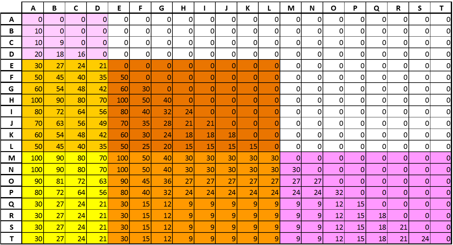
Table 7.10Station Saturation at Example Corridor for Tenth Year with One Limited-Stop Service
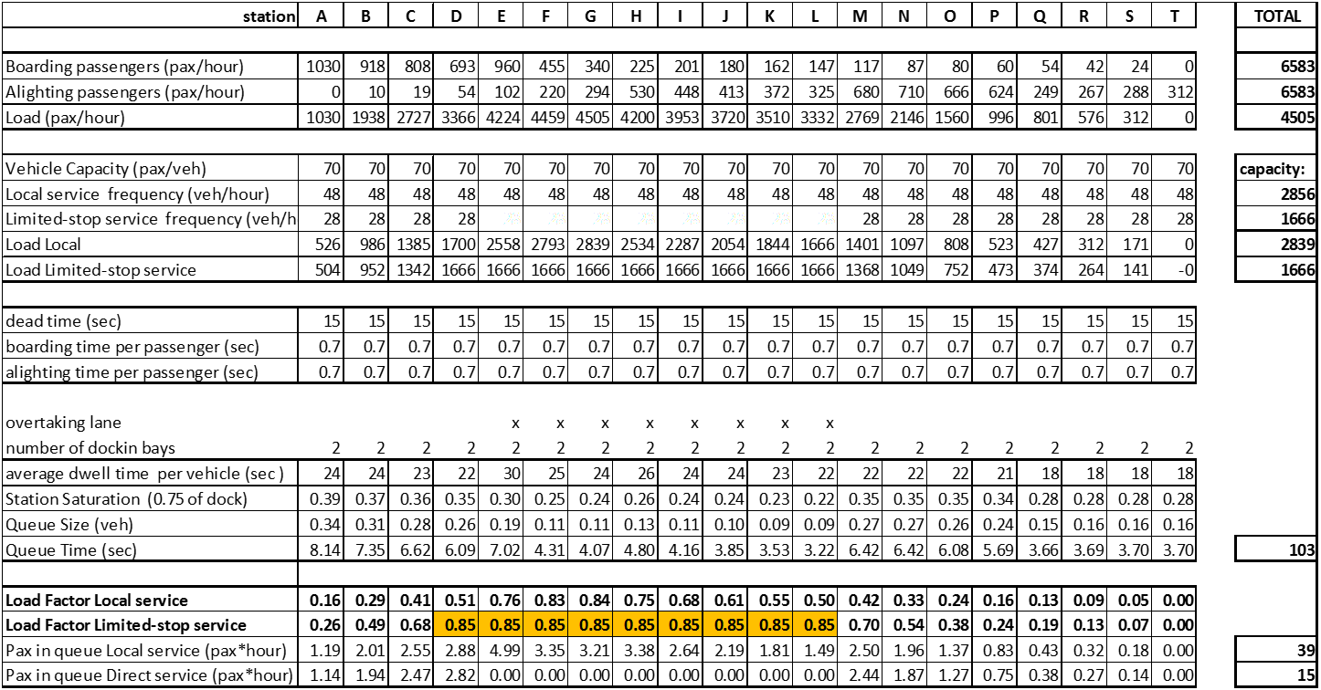
The additional queue waiting time in relation to the previous alternative is forty seconds, but after the addition of the limited service, the travel time difference between local and limited stop is only twenty-six seconds, which would end up making no difference for users who can take the limited service to use that route. If customers could be forced to behave the way we assumed, the total queueing time would be further reduced from eighty-three to fifty-five. To force this behavior, one can propose, in addition to the limited service, to split the local service into two early return services: the first (Local 1) would attend from station A to station L, and the second (Local 2) from station E to station T.
Passengers shown in the OD matrix would have the options below:
- Light pink: Local 1 or Limited-stop
- Light orange: Local 1
- Yellow: Limited-stop
- Brownish orange: Local 1 or Local 2
- Medium orange: Local 2
- Darker pink: Limited-stop or Local 2
When splitting the original local in two, splitting the original frequency (48 vehicles per hour) is not enough to serve the loads between stations D and E and stations L and M, so the sum of frequencies of this new service (28.5 and 23.1) ends up being higher than the original alternative. Total travel time before the split was 25.6 vehicle-hours (during the peak hour), and after it became 19.2 vehicle-hours, indicating a potential fleet reduction. If a reversion time of five minutes on each side is considered, a symmetrical return and a constant demand (PHtoCC = 0), instead of needing sixty vehicles, only forty-eight are needed to run the local service.
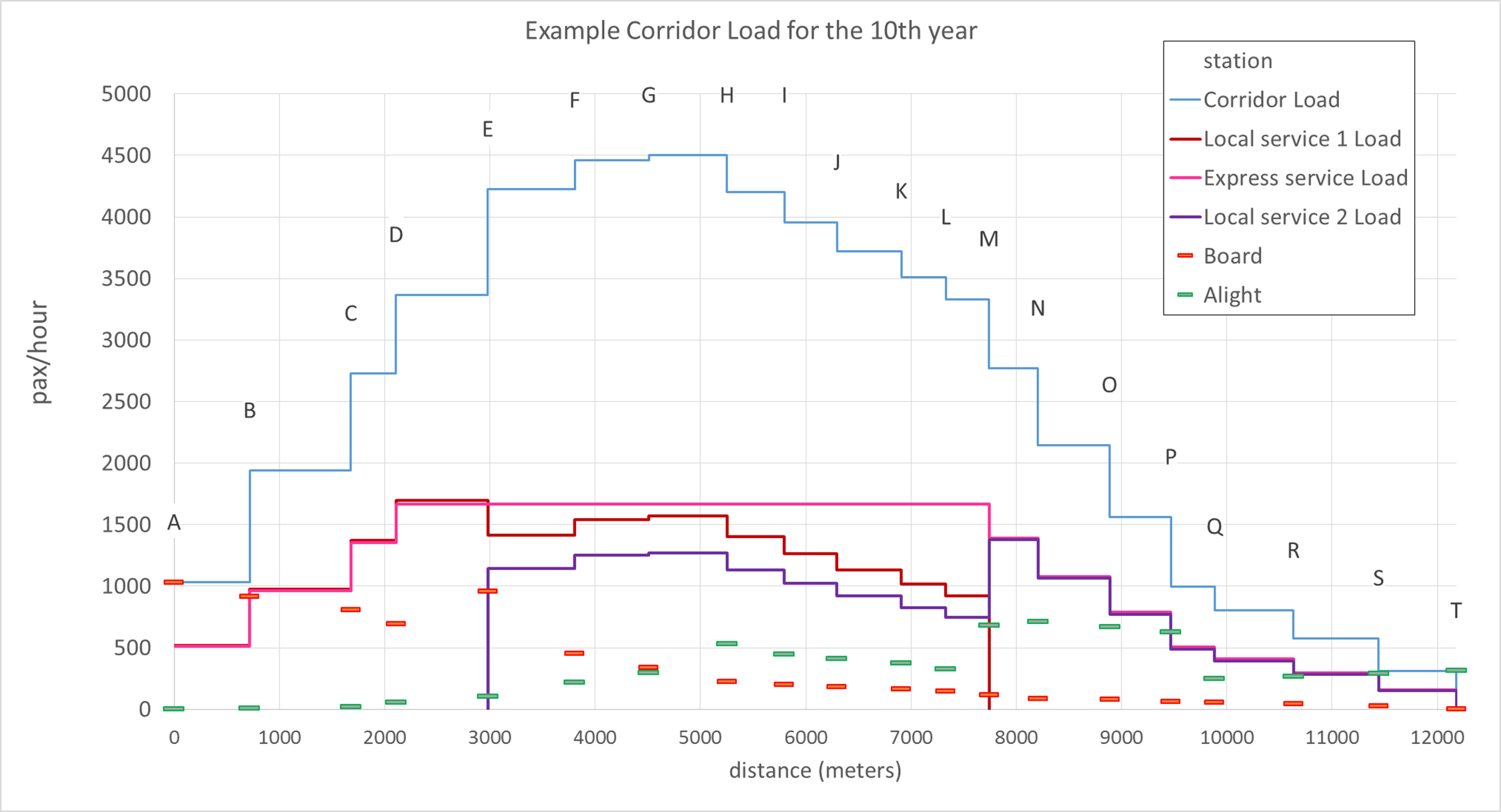
Besides that, as shown in Table 7.11, there is some meaningful reduction in saturation for stations from A to D and M to T while the stations E to L face a small increase. Passenger time in queue is further reduced to fifty hours, against eighty-three without overtaking lanes and direct service. Figure 7.8 shows the resulting loads in each service.
Table 7.11Station Saturation at Example Corridor for Tenth Year with Limited and Early Return Local Services