7.2The Process of Designing High-Capacity and High-Speed BRT Corridors

7.2.1Concepts Review

One can reasonably expect that capacities are independent of demand — that once the specifications of design and operation are given, the capacity could be calculated regardless of the demand. This is true for each feature of BRT, but there are so many possible limitations to these features that a global analysis without restricting them to the intended use has no practical purpose. Consider the analogy of a truck’s capacity (or a glass mug’s, as in Figure 7.3): maximum volume, maximum weight, and maximum dimensions are clearly defined, but discussing capacity without knowing what will be transported — cotton, steel, or windmill blades—leaves too many possibilities open. Similarly, given an elevator design — load, speed, door opening times, and protocol to answer calls — one can simulate the wait and travel times for a given demand pattern, but to evaluate all of them would be impractical. It is much easier to evaluate the capacity for a given use.

For this edition, we changed the approach for calculating operational capacity of a corridor: the capacity of the corridor is the capacity of its bottleneck One must evaluate the capacity of each station and traffic lights under predicted conditions to check the corridor capacity.

In order to compare situations for design, capacity is defined as the number of customers that can pass through a given cross section during a time interval. For practical purposes, we will examine that cross section for one-way traffic only and use one hour as a reference measure for the interval.

The capacity of a segment (or link) should be given by the lower capacity of a section within it (lower capacity section along the segment). Unlike intersections, where the stop line can be readily identified as the bottleneck of the approaching segment, BRT stations with multiple sub-stops are harder to model as single session; they are easier seen as segments which will have still many potential sections to evaluate for discovering the lower-capacity section. Anyway, the capacity is the maximum possible load across the station.

Further confusion could arise by considering the station as a segment, because the load entering the station is not the load leaving the station, unlike a traditional demand segment or link in modelling that is between stations. But that is not a problem for calculating capacity because we are considering the maximum possible load. When dealing with demand load, every demand load in the system would still be taken into account because the load that leaves one station arrives at the next. For the purposes of calculating capacity here, the demand load of a station is the demand load that arrives at it.

As mentioned before and as will be highlighted many times in the following discussions and examples, high capacity is achievable at the cost of speed. Therefore, in agreement with our design objectives, we define the operational capacity as the capacity that does not cause bus queues at the stations.

What constitutes a queue is still a bit subjective and will be discussed when queue formation is evaluated. One should notice that having no queue does not necessarily imply reduced time at the station. For example, one station in a well-designed system could have a boarding and alighting process taking one minute regularly every five minutes (20 customers boarding through a stepped door), and that would be a fine operation with low operational capacity, which will also be shown later in the chapter.

This definition of capacity is not the capacity of the station itself, but the capacity of the corridor segment where the station is. The station itself has other capacities that need to be specified (or calculated for a given design), including:

• Number of waiting customers, which varies based on comfort parameters;
• Number of boardings per hour and number of alightings per hour, which may be given by a curve when one is dependent of the other (i.e., they use the same door).

More information on station design can be found in Chapter 25: Stations.

The renovation rate is an important concept for understanding that the total number of customers transported by a route may be higher than the capacity of the route as usually defined (it can be lower, too, but that is not difficult to understand). The same concept is needed to evaluate the BRT corridor: the number of customers using the system may be higher than its capacity.

Another observation must be made regarding the renovation rate: when operators and business analysts mention it, they normally refer to transported customers (in a trip, route, or corridor) over the effective supply (the capacity of the vehicles providing the service—trip-places), ignoring both the load factor required for appropriate planning and the fact that in the first years of operation the supply is often lower than capacity, because corridors need to be designed for higher capacity than existing demand, and thus, supply.

One must keep in mind that transport systems’ speeds, waiting times, supplied trip-places, demand, and maximum loads will change throughout the day, throughout the seasons, and throughout the years. By monitoring operational data of a built system, one can certainly tell the lower bounds of its capacity (capacity will certainly be greater or equal to the maximum load observed), but even so, the operational capacity would be subject to debate.

7.2.2Simulating Solutions

Regardless of the debate about operational capacities of transport systems, it is very simple to evaluate the capacity and speed of a proposed design solution under any condition and compare it with other solutions and conditions, including using a car. Besides understanding how to compute dwell time and queuing time in stations, which will be discussed in this chapter, and at traffic lights, which will be discussed in Chapter 24: Intersections and Traffic Signals, the basic requirement is manipulation of the cinematic concept of speed.

Speed is useful to bringing users travelling different distances to a common location, but for evaluation of the system, only the use of speed for evaluation is necessary because people, including planners in and stakeholders of the project, are familiar with speeds, knowing the sensation of movement associated with the readings in a speedometer of a car. A planner compares alternatives of the same implementation and operational cost by comparing the sum of travel times for all people in the city (both those using and not using the system) with the implementation of each alternative.

That said, the equations needed to simulate and compare speeds are:

\[ \text{average speed} ={\text{travel distance} \over \text{travel time} } \leftrightarrow \text{travel time} = {\text{travel distance} \over \text{average speed}} \]

\[ \text{travel time}_{A-Z} = \text{travel time}_{A-M} + \text{wait time}_M + \text{travel time}_{M-Z} \]

The last equation assumes point M is part of travelling itinerary between points A and Z. It can be further divided, assuming that point B is between points A and M.

\[ \text{travel time}_{A-M} = \text{travel time}_{A-B} + \text{wait time}_B + \text{travel time}_{B-M} \]

This implies the obvious understanding that the travel time along a corridor is the sum of travel time in every segment (or link) with the wait time at every stopping point.

A simple table like Table 7.1 can be constructed to compare travel time and speed for different alternatives and conditions.

Table 7.1Example of Travel Time Simulation under Different Conditions

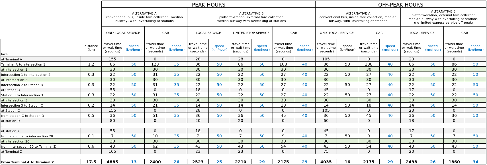
This table can be placed in a different order, joining the unshaded rows (segment times), green shaded rows (intersection times), the gray shaded rows (station times) and programmed to calculate each value based on the characteristics of the proposed design and operation based on the following formulas of this chapter for stations, the formulas given in Chapter 24: Intersections and Signal Control, and in the basic speed formula given for segments. In the initial planning phases, assumptions for intersections plus segments based on observed travel times are good enough for a practical evaluation of alternatives.

A similar table (as shown in Table 7.1) can be made for the capacity of each section, once formulas for capacity are given for stations in the remainder of the chapter, and formulas for capacity of segments, and intersections are given in Chapter 24, based on the proposed design characteristics.

So, with the forecast demand and the design, one can tell if the required performance, initially taken as an assumption, is reached. If not, modifications need to be proposed for the infrastructure (or technology) where failure was observed in relation to expected results. In the unlikely case that an excessive performance is seen, adjustments could also be proposed for a more adequate system. For both cases, the last two sections of this chapter (7.5 and 7.6) will discuss how station, vehicle, and operation features affect speed and capacity.

The next section (7.3) explains how the station design associated with the service plan affects system speed and the following (Section 7.4) discusses how the design of the station for a given boarding and alighting demand affects system capacity.