7.3Understanding Station Saturation

How did it get so late so soon? It’s night before it’s afternoon. December is here before it’s June. My goodness how the time has flewn. How did it get so late so soon?Theodor Seuss Geisel (aka “Dr. Seuss”), writer and cartoonist, 1904–1991

If the highest frequency at a BRT corridor bottleneck is one bus per minute, the rest of the corridor will have at most a one bus per minute frequency. Identifying this weak link in the system is the foundation for improving capacity and avoiding congestion, which in turn improves travel times. In general, the critical factor on a public transport system is vehicle congestion at the station.

The fact that BRT systems are now able to reach speeds and capacities comparable to all but the highest capacity metro systems is due to dramatic improvements in vehicle capacity at stations. Other factors are also important to reaching these speed and capacity goals, but none are as important as preventing docking bay congestion. Many existing BRT systems are burdened with slow operating speeds due to incorrect demand projections at particular stations. Poorly designed stations can lead to peak-hour vehicle queues that stretch for several hundred meters.

The proper design of a station to prevent congestion is directly related to the concept of saturation level, usually referred to simply as saturation.

The saturation level of a docking bay refers to the proportion of time that a vehicle docking bay is occupied. A docking bay is the designated area in a BRT station where a vehicle will stop and align itself to the boarding platform.

A docking bay might be considered occupied at any given moment, if a bus that wants to position itself at that docking bay cannot proceed with the proper maneuver. Therefore, a vehicle is “using” the docking bay from the moment its approach will prevent other vehicles from doing the same thing until the moment it leaves the area so that another vehicle can approach. The amount of time that any given vehicle occupies a docking bay is called dwell time (\(T_d\)).

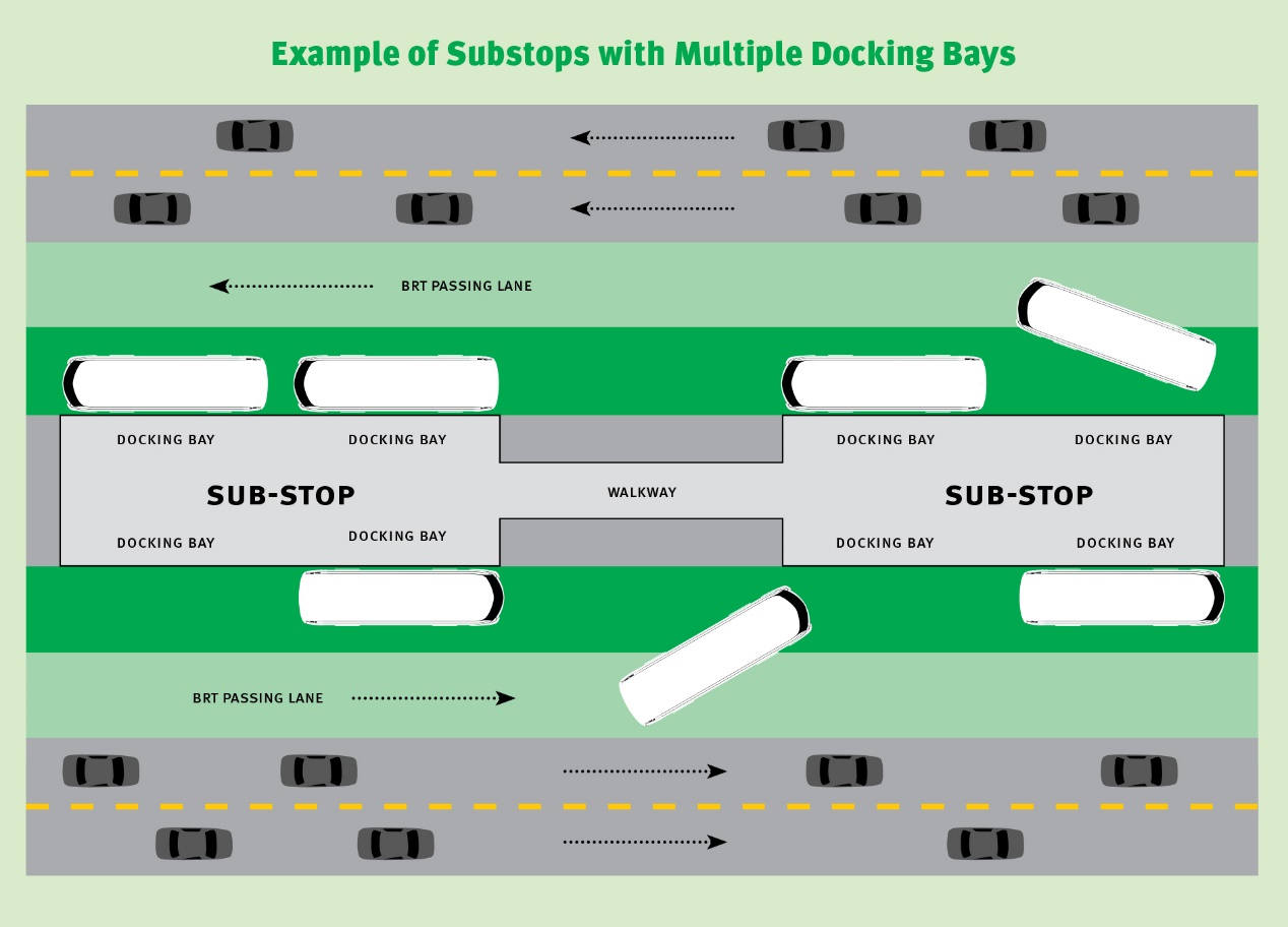
Box 7.1 Sub-Stops and Docking Bays

A schematic view of a station, from The BRT Standard, shows the components of a station including the sub-stops and the docking bays, defined as follows:

• Sub-stop: a station subdivision or “module” that includes docking bays and customer circulation and waiting areas. One station can have multiple sub-stops that are physically connected. In order for multiple sub-stops to function, they typically need overtaking lanes or a functional equivalent such as in the “directional” BRT stations used in Lanzhou and Yichang.
• Docking bay: the platform-vehicle interface; this is where the bus pulls up in order to let customers on and off.

Therefore, the saturation of a docking bay (\( x_dock \)) measured for a certain time interval (\( \Delta t \)) would be given by the sum of dwell times of each bus docking (\( Ti di \)) during that interval, divided by the duration of the interval, as expressed by Equation 7.1.

Eq. 7.1 Saturation of a docking bay concept:

\[ x_\text{dock} = {\sum_{\text{docking bus} i \in \Delta t} {T}_{i d} \over \Delta t} \]

Where:

• \( x_\text{dock}\): Saturation of a docking bay;
• \( \sum_{\text{docking bus} i \in \Delta t} {T}_{i d} \): Sum of docking times of buses;
• \( \Delta t\): Time interval.

Calling \(T_d\) the average dwell time (which is equivalent to assuming that all buses will have the same dwell time \(T_d\)), saturation would be:

\[ x_\text{dock} = {N_{\text{buses} \in \Delta t} * {T}_{i d} \over \Delta t} \]

And calculating the saturation for one hour would result in the following equation:

Eq. 7.2 Saturation of a docking bay for one hour:

\[ x_\text{dock} = {Freq_\text{dock} * T_d \over 3600\text{sec}} \]

Where:

• \( x_\text{dock} \): Saturation of a docking bay;
• \( \text{Freq}_\text{dock} \): Frequency of buses docking;
• \( T_d \): Dwell time.

The dwell time consists of three separate categories: boarding time, alighting time, and dead time. Boarding and alighting times can partially happen simultaneously, depending on the system protocol for boarding and alighting. Dead time is the time consumed by a vehicle slowing down when approaching a station, opening its doors (and after a variable dwell time for boarding and alighting), closing its doors, and then regaining free flow speed. It is also called fixed dwell time because it is the part of dwell time that does not vary with the number of customers boarding and alighting at each stop, and it usually does not vary between stops in a system.

Two elements of the BRT vehicle affect dead time: the rate of vehicle deceleration when approaching a stopping bay and the rate of acceleration when departing from a docking bay. Besides the vehicle capabilities (power-to-weight and gear relations), the deceleration and acceleration rates often involve a trade-off between speed and customer comfort, as well as the ability to properly align the vehicle to the stopping-bay interface.

Vehicle size also affects the dead time. In non-congested situations, vehicles typically require ten to sixteen seconds to open and close their doors and pull in and out of a station and, when in a queue, up to twenty seconds. However, larger vehicles require more time, and additional time between 0.17 to 0.25 seconds per meter of vehicle is generally required for pulling in and out of the station. For a more detailed model, these values need to be calibrated to produce the amount of dead time, but as a conservative approach Equation 7.3 can be used.

Eq. 7.3 Impact of vehicle length on dwell time without queue

\[ T_0 = 13 + L_\text{vehicle} * 0.25 \]

Where:

• \( T_0\): Dead time in seconds;
• \( L_\text{vehicle}\): Length of the vehicle in meters.

As for the variable part of dwell time (boarding and alighting time), the main factors affecting it include:

• Customer-flow volumes;
• Number of vehicle doorways;
• Width of vehicle doorways;
• Entry characteristics, e.g., stepped or at-level entry, using all doors or having specific doors to board and alight;
• Open space near doorways (on both vehicle and station sides);
• Fare collection position, e.g., at the station entrance, at the bus entrance, in the middle of the bus;
• Doorway control system.

BRT systems are able to operate metro-like service in large part due to the ability to reduce total stop time to twenty seconds or less. A conventional bus service often requires more than sixty seconds for stop time, though the specific time will be a function of the number of customers and other factors. In general, dwell times may be somewhat higher during peak periods than nonpeak periods. The increase during peak periods is due to the additional time needed to board and alight the higher customer volumes.

In a system where both boarding and alighting happens through all doors, dwell time is given by Equation 7.4:

Eq. 7.4 Dwell time for one bus with an external fare collection and all-door boarding: \( T_d =T_0 + p_b * t_b + p_a * t_a \)

Where:

• \( T_d \): Dwell time for a given bus;
• \( T_0 \): Dead time for the given bus;
• \( t_b \): Average boarding time per customer;
• \( t_a \): Average alighting time per customer;
• \( p_b \): Number of boarding customers at the given bus;
• \( p_a \): Number of alighting customers at the given bus.

If boarding is made exclusively through different doors than alighting, then the dwell time for a bus is given by Equation 7.5:

Eq. 7.5 Dwell time for one bus with specific doors for boarding or alighting:

\[ T_d = T_0 + Max(p_b *t_b,p_a * t_a) \]

Where:

• \( T_d \): Dwell time for a given bus;
• \( T_0 \): Dead time for the given bus;
• \( t_b \): Average boarding time per customer;
• \( t_a \): Average alighting time per customer;
• \( p_b \): Number of boarding customers at the given bus;
• \( p_a \): Number of alighting customers at the given bus.

Equation 7.6 shows the saturation calculation for the situation where both boarding and alighting occur through the same doors.

Eq. 7.6 Calculating the saturation level of a docking bay for a given time interval, under external fare collection and all door boarding:

\[ x_\text{dock} = {T_0 * N_\text{bus} + [ (P_b * t_b) + (P_a *t_a) ] \over \Delta t} \]

Where:

• \( x_\text{dock} \): Saturation level of a docking bay for a given time interval;
• \( N_\text{bus} \): Number of vehicles that use the docking bay during the interval (if the time interval is an hour it is the usual frequency of services referenced in vehicles per hour);
• \( T_0 \): Average dead time per bus;
• \( t_b \): Average boarding time per customer;
• \( t_a \): Average alighting time per customer;
• \( P_b \): Number of boarding customers at docking bay during interval;
• \( P_a \): Number of alighting customers at docking bay during interval;
• \( \Delta t \): Time interval duration (this is usually seen as 3,600 since one hour calculation is normally done and other times are given in seconds).

The equation shows that for a given demand (number of customers) using a docking bay to board and alight, the way to reduce saturation is by minimizing the time needed to board or alight or by reducing the number of buses, given that the dead time cannot be significantly reduced. The remaining alternative is to split the demand in more docking bays.

To illustrate the saturation calculation, we take the example of a TransMilenio’s, Modulo A2 of Alcalá Station (March 8, 2007, data) where between 7:00 a.m. and 8:00 a.m. there were 62 vehicles stopping, 975 boarding customers, and 23 alighting customers. The dead time is 15 seconds, boarding time per customer is 0.3 seconds, and alighting time per customer is 0.2 seconds. This way, the saturation level between 7:00 a.m. and 8:00 a.m. can be estimated as:

\[ x = {15 {\text{sec} \over \text{vehicle}} * 62 \text{vehicles} +[( 975 \text{pax} * 0.3{\text{sec} \over \text{pax}}) + (23 \text{pax} * 0.2 {\text{sec} \over \text{pax}})] \over 3,600 \text{sec}} \]

\[ x = {930 \text{sec} + [(292.5 \text{sec}) + (4.6 \text{sec})] \over 3,600 \text{sec}} = {409 \text{sec} \over 3,600 {sec}} = 0.11 \]

Understanding saturation is important because queue formation is a function of it.

According to the theory of queues, the expected queue a vehicle faces when approaching a station would be given by Equation 7.7

Eq. 7.7 Queue size:

\[ \text{QueueSize}_\text{dock} = { 0.5 * (Irr_\text{arrival}+ Irr_\text{departure})* x_\text{dock} ^ 2 \over (1-x_\text{dock})} \]

Where:

• \( \text{QueueSize}_\text{dock} \): Average or expected queueing size at docking bay;
• \( x_\text{dock} \): Saturation level of a docking bay for a given time interval; xdock = Saturation of a docking bay;
• \( Irr_\text{arrival} \): Irregularity of arrivals (\(= {\text{Variance}_\text{arrivals' intervals} \over \text{Mean}_\text{arrivals' intervals} ^2 } \));
• \( Irr_\text{departure} \): Irregularity of departures (\(= {\text{Variance}_\text{departures' intervals} \over \text{Mean}_\text{departures' intervals} ^2 } \)).

The mean of the intervals for arrivals and departures is the headway, and the variance would be similar to the variance for boardings and alightings if there were no traffic lights and starting schedules were exactly followed. If a service was totally regular, no queues would be expected. The particular case when irregularities for arrival and departure are random (\( Irr_\text{arrivals} = Irr_\text{departures} = 1 \)) would result in the queue given by Equation 7.8.

Eq. 7.8 Queue size for random arrivals and random boarding-alighting times (the mean can be known):

\[ \text{QueueSize}_\text{dock} = { x_\text{dock} ^ 2 \over (1-x_\text{dock})} \]

Where:

• \( \text{QueueSize}_\text{dock} \): Average or expected queueing size at docking bay;
• \( x_\text{dock} \): Saturation level of a docking bay for a given time interval.

For the common irregularities observed in urban busways with high volumes (headways below one minute), Equation 7.9, derived from observation, can be used:

Eq. 7.9 Queue size for busways in typical urban conditions:

\[ \text{QueueSize}_\text{dock} = { { 0.7 * x_\text{dock}^2} \over (1-x_\text{dock})} \]

Where:

• \( \text{QueueSize}_\text{dock}\): Average or expected queueing size at docking bay;
• \( x_\text{dock}\): Saturation level of a docking bay for a given time interval.

The expected (average) waiting time in queue (\(T_\text{queue}\)) is given by the queue size multiplied by the average headway, as expressed in Equation 7.10:

Eq. 7.10 Time waiting in queue:

\[ T_\text{queue} = \text{QueueSize} * \text{Hdwy} \]

Where:

• \( T_\text{queue} \): Time waiting in queue;
• \( QueueSize \): Average or expected queueing size;
• \( \text{Hdwy}:\) Average headway.

A low saturation level or a high level of service means that there are no vehicles queuing at a docking bay. A high saturation level means that there will be long queues at docking bays. Therefore, increasing station saturation tends to lead to a gradual deterioration of service quality. For saturation levels over one (\( x > 1 \)), the system is unstable with queues increasing until the demand is reduced after the peak period.

For the previous example, the module of Alcalá station has a low saturation rate (0.11). At this level, one should not expect to have congestion problems at the station, as the expected queue size and time would be irrelevant:

\[ \text{QueueSize}_\text{dock} = { { 0.7 * x_\text{dock}^2} \over (1-x_\text{dock})} = { 0.7 * 0.11^2 \over (1-0.11) } = 0.0095 \]

\[ T_\text{queue} = \text{QueueSize} * \text{Hdwy} = 0.0095 \text{vehicles} * {1 \over 62 {\text{vehicles} \over \text{hour}}} = 0.00153 \text{hour}= 0.55 \text{sec} \]

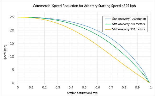
The decision about which saturation levels can be tolerated in specific locations should be considered within the overall design context. However, one must keep in mind that for saturation levels above 0.60 (or 60 percent), the risk of severe congestion and system breakdown is considerable. For BRT stations, 40 percent is the maximum accepted for planning purposes, allowing a reasonable safety margin for uncertainties in the planning process. That is, the cumulative time that a vehicle is stopped at a station should not exceed 40 percent of the total time available in an hour.

Expected station saturation effects on commercial speeds are shown in Figure 7.5. Bogotá’s TransMilenio strives to keep the saturation value in the range of 0.35 to 0.45. The Calle 76 station of the TransMilenio system illustrates the importance of accurately projecting customer movements and station saturation levels. Originally, this critical station was planned for a saturation level of 0.40, but during actual operation the saturation reached 0.65 due to an unexpectedly high number of transfers. Similar levels of saturation were experienced at Heroes Station (which has subsequently been expanded), where saturation was much higher than the 0.40 level anticipated. This experience shows the importance of being somewhat conservative by planning for 40 percent station saturation.

When boarding is made through different doors, one could expect saturation to be calculated as given by Equation 7.11.

Eq. 7.11 Simplified saturation level of a docking bay where boarding is through specific doors:

\[ x_\text{dock} = {T_0 * N_\text{bus} + Max(p_b *t_b,p_a * t_a) \over \Delta t} \]

Equation 7.11 works when one of the movements between boarding and alighting is clearly longer or if customers arrive at stations in a completely regular fashion between the bus passages (the longer the headway the more regular this number is). But if the times for boarding and alighting are similar, then there will be a certain number of times when boarding will end first and a certain number of times when alighting will end first. If the expected times for each operation were equal, then each operation would be expected to end first half of the time.

For a random distribution of boarding and alighting times (where the average times are known), the number of occasions that the one operation will be longer than the other is given by Equation 7.12.

Eq. 7.12 Expected occurrence of the shortest time overcoming the longer:

\[ rf1 = {\overline{t1} \over \overline{t1} + \overline{t2}}\]

Where:

• \( rf1 \): Relative frequency where event 1 is longer than event 2;
• \( \overline{t1} \): Average length of distribution of events 1;
• \( \overline{t2} \): Average length of distribution of events 2;

Using the Poisson distribution, a discrete probability distribution, for events 1 and 2, where the standard deviation is equal to the mean, is assumed.

If we call the mean boarding time per bus of \( T_b \), with \( T_b = t_b * P_b \), and mean alighting time per bus of \( Ta \), with \(T_a = t_a * p_a \), the average dwell time would be given by Equation 7.13.

Eq. 7.13 Saturation level of a docking bay where boarding is through specific doors:

\[ T_d = T_0 + T_a + ({T_b \over T_a + T_b}) * T_b = T_0 + T_b + ({T_a \over T_a + T_b}) * T_a \]

Where:

• \( T_d \): Average dwell time for all buses on a docking bay;
• \( T_o \): Average dead time for all buses on a docking bay;
• \( T_a \): Average alighting time for all buses on a docking bay;
• \( Tb \): Average boarding time for all buses on a docking bay;
• \( T_b \over T_a + T_b \): Relative frequency that boarding will be longer than alighting;
• \( T_a \over T_a + T_b \): Relative number of times that alighting will be longer than boarding.

Therefore the saturation for a docking bay where boarding is made through specific doors is given by Equation 7.14.

Eq. 7.14 Saturation calculation when boarding is through a specific door:

\[ x_\text{dock} = {T_0 * N_\text{bus} + P_b * t_b + ({P_a * t_a \over P_a * t_a + P_b * t_b}) * P_a * t_a \over \Delta t} \]

Where:

• \( x_\text{dock} \): Saturation level of a docking bay for a given time interval;
• \( N_\text{bus}: \): Number of vehicles that use the docking bay during the interval (if the time interval is an hour it is the usual frequency of services referenced in vehicles per hour);
• \( T_0 \): Average dead time per bus;
• \( t_b \): Average boarding time per customer;
• \( t_a \): Average alighting time per customer;
• \( P_b \): Number of boarding customers at docking bay during interval (average boarding time per bus is given by \( T_b = t_b * P_b \));
• \( P_a \): Number of alighting customers at docking bay during interval(average alighting time per bus is given by \( T_a = t_a * P_a \);
• \( \Delta t \): Time interval duration (this is usually seen as 3,600 since one hour calculation is normally done and other times are given in seconds).

For example, a regular bus stop in front of a children’s hospital in São Paulo, using data from between 6:00 a.m. and 7:00 a.m. on February 2, 2007, is served by two routes with a frequency of four trips per hour each. The average number of boardings per vehicle is 4.1, for a total of 33, and the average number of alightings per vehicle is 10, for a total of 80. People carrying babies count as one. The average time per person for boarding is five seconds, and for alighting it is three seconds, with one wheelchair alighting taking around forty-five seconds. The saturation of this stop would be calculated as:

\[ x_\text{dock} = {T_0 * N_\text{bus} + P_b * t_b + ({P_a * t_a \over P_a * t_a + P_b * t_b}) * P_a * t_a \over \Delta t} \]

\[ x = {16 {\text{sec} \over \text{vehicle}} * 8 \text{vehicles} +( 33 \text{pax} * 5 {\text{sec} \over \text{pax}}) + ({80*3.0 \over 80*3.0 +33*5}) * 80 \text{pax} * 3.0 {\text{sec} \over \text{pax}} \over 3,600 \text{sec}} \]

\[ x = {128 \text{sec} + (165 \text{sec}) + ({240 \over 240 + 165}) * 240 \text{sec} \over 3,600 \text{sec}} \]

\[ x = {128 \text{sec} + (165 \text{sec}) + ({240 \over 405}) * 240 \text{sec} \over 3,600 \text{sec}} \]

\[ x = {128 \text{sec} + (165 \text{sec}) + 0.59 * 240 \text{sec} \over 3,600 \text{sec}} = 0.12 \]

With the stop being occupied only 12 percent of the time, the average expected queue is 0.012 (each hundred arrivals the stop will be used by another bus), and the average queue delay is 5 seconds, as calculated below:

\[ \text{QueueSize} = { 0.7 * x_\text{dock}^2 \over (1-x_\text{dock})} = { 0.7 * 0.12^2 \over (1-0.12) } = 0.0116 \]

\[ T_\text{queue} = \text{QueueSize} * \text{Hdwy} = 0.0116 \text{vehicles} * {1 \over 8 {\text{vehicles} \over \text{hour}}} = 0.001455 \text{hour}= 5.23 \text{sec} \]

7.3.1Saturation on a Sub-Stop with Many Docking Bays

The defining characteristic of a sub-stop with two or more docking bays is that a vehicle can leave the sub-stop only if the vehicle in front of it has already left. We can assume that if this design is under consideration, the saturation for only one docking bay is relatively high, so we may ignore the situations where frequency is low and dwell times are short. We are facing something between two extreme situations:

• Low frequencies with many customers boarding and alighting in a terminal-like situation;
• High frequencies with short dwell time.

Of course, another situation could be when there is a high boarding-alighting demand with high service frequencies without the use of overtaking lanes.

Same service at all docks

If the vehicles that dwell at the sub-stop with N docking bays were all serving the same route and the vehicles were riding in a platoon (of N vehicles), this would be equivalent to having a longer vehicle (like a train): the number of doors would be multiplied by N, both the boarding time and the frequency of this longer vehicle would be the original frequency divided by N too, which in this case, saturation would be divided by N.

That is ignoring that the dead time for the “train” would be slightly longer than that of one vehicle alone; this difference would not be meaningful considering the lack of precision in the previously proposed Equation 7.3 when there is no queue.

But when the bay is congested (i.e., is a queue moving), which is the likely situation when multiple docking bays are under consideration, the dead time for the whole convoy would be given by Equation 7.15.

Eq. 7.15 Dead time for convoy:

\[ T_{0\text{convoy}} = 13 + 0.25 * L_\text{vehicle} * 0.25 + (2 + 0.17 * L_\text{vehicle}) * (N - 1) \]

Where:

• \( T_{0 convoy}\): Dead time in seconds for the whole convoy;
• \( N \): Number of vehicles in the convoy;
• \( L_\text{Vehicle} \): Length of each convoy vehicle in meters (average vehicle length when vehicles are different).

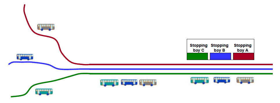
Ordered platoon (routes attributed to docks)

If the routes stopping at the sub-stop are different, but platoons are organized when entering the busway (Figure 7.6) always in an order that customers can be positioned on the platform in front of the right docking bay, the whole “train” would leave the station once boarding and alighting in the most heavily demanded “car” was completed.

If the number of arrivals of customers at the station was regular and equally distributed at all routes, the saturation for the sub-stop would be equal to the saturation of the most congested docking bay, when an average queue size is N times bigger.

But if the number of customers that arrive at a station to board each route is variable, then an additional dwell time must be added to calculate the saturation of the most congested docking bay. To do this, within that variability, there is an expected regularity, with the known mean and equal standard deviation value of the worst case. This is a situation similar to boarding and alighting through different doors, as at certain times the boarding-alighting times of each platform may overcome the others.

Assuming \(T_{i b/a}\) is the average boarding and alighting time calculated for the ith docking bay, if there were two docking bays, the average dwell time for the convoy would be given by Equation 7.16.

Eq. 7.16 Average dwell time for two docking bays in a sub-stop:

\[ T_\text{d 2 bays} = T_0 + T_1 + T_2 - {1 \over {1 \over T_1} + {1 \over T2}} = T_0 + T_1 + {T_2 \over T1+T2 } * T2 \]

If there are three platforms, the equation (shown in 7.17) gets a bit longer.

Eq. 7.17 Average dwell time for three docking bays in a sub-stop:

\[ T_\text{d 3 bays} = T_0 + T_1 + T_2 +T_3 \]

\[ - {1 \over {1 \over T_1} + {1 \over T2}} - {1 \over {1 \over T_1 } + {1 \over T3}} - {1 \over {1 \over T_2 } + {1 \over T3}} \]

\[ + {1 \over {1 \over T_1 } + {1 \over T_2 } + {1 \over T3}} \]

For four platforms it gets even longer and becomes too impractical and difficult to apply.

Eq. 7.18 Average dwell time for four docking bays in a sub-stop:

\[ T_\text{d 4 bays} = T_0 + T_1 + T_2 + T_3 + T_4 \]

\[ - {1 \over {1 \over T_1} + {1 \over T2}} - {1 \over {1 \over T_1} + {1 \over T3}} - {1 \over {1 \over T_1} + {1 \over T4}} - {1 \over {1 \over T_2} + {1 \over T3}} - {1 \over {1 \over T_2} + {1 \over T4}} - {1 \over {1 \over T_3} + {1 \over T4}} \]

\[ + {1 \over {1 \over T_1} + {1 \over T_2} + {1 \over T3}} + {1 \over {1 \over T_1} + {1 \over T_3} + {1 \over T4}} + {1 \over {1 \over T_2} + {1 \over T_3} + {1 \over T4}} \]

\[ - {1 \over {1 \over T_1} + {1 \over T_2} + {1 \over T_3} + {1 \over T4}} \]

Where:

• \( T_\text{d N bays} \): Average dwell time for a sub-stop with N docking bays (equation will have \(2^N \) terms);
• \( T_0 \): Dead time (given by Equation 7.15);
• \( T_i \): Variable dwell time for ith docking bay calculated in isolation (given by Equation 7.4 or 7.13 minus \( T_0\)).

This equation can be extended to any number of platforms and can be relatively easily implemented by an algorithm, but an alternative formula (Equation 7.19) that underestimates saturation by 2 percent for each additional docking bay above two can be used for practical purposes.

Eq. 7.19: Practical approximation for average dwell time for N docking bays in a sub-stop:

\[T_\text{d N bays}: T_0 + {3 \over N + 2} * \sum_{i=1} ^N {T_i} \]

Where:

• \( T_\text{d N bays}\): Average dwell time for a sub-stop with N bays (equation will have 2N terms);
• \( N \): Number of vehicles in the convoy;
• \( T_0 \): Dead time (given by Equation 7.15);
• \( T_i \): Variable dwell time for ith docking bay calculated in isolation (given by Equation 7.4 or 7.13 without considering \(T_\text{0}\) there).

Unordered vehicles

If the routes stopping at the sub-stops are different and may arrive in any order, the approximation for saturation is the same, but what is observed in reality is that for sub-stops with three or more docking bays, a certain quantity of vehicles stops twice to pick up customers that miss the vehicle dwelling at the first time. Unless there is operational enforcement for preventing this second stop, this can be seen as enforcing bad service.

In a design situation, more than three docking bays without organized convoys should not be proposed. If dealing with an existing situation, the safest thing to do is to measure the existing saturation.